RENAULT TECHNOLOGIE ROUMANIE Dr. Ioan TELEAGA Brasov, june 2011 DINAMICA FLUIDELOR COMPUTATIONALA APLICATA LA VEHICULE: DE LA TEORIE LA PRACTICA Profesionalism şi exemplaritate Respect şi solidaritate Dezvoltare personală Satisfacţia clientului Valorile RTR
Transcript
RENAULT TECHNOLOGIE ROUMANIEDr. Ioan TELEAGA Brasov, june 2011
DINAMICA FLUIDELOR COMPUTATIONALA APLICATA LA VEHICULE: DE LA TEORIE LA PRACTICA
Profesionalism şi exemplaritate
Respect şi solidaritate
Dezvoltare personală
Satisfacţia clientului
Valorile RTR
RENAULT TECHNOLOGIE ROUMANIEDr. Ioan TELEAGA Brasov, june 2011 2
Overview
INTRODUCTION
01FROM THEORY TO
NUMERICS
02AERODYNAMICS
03THERMODYNAMICS
04
RENAULT TECHNOLOGIE ROUMANIEDr. Ioan TELEAGA Brasov, june 2011
01 INTRODUCTION
RENAULT TECHNOLOGIE ROUMANIEDr. Ioan TELEAGA Brasov, june 2011
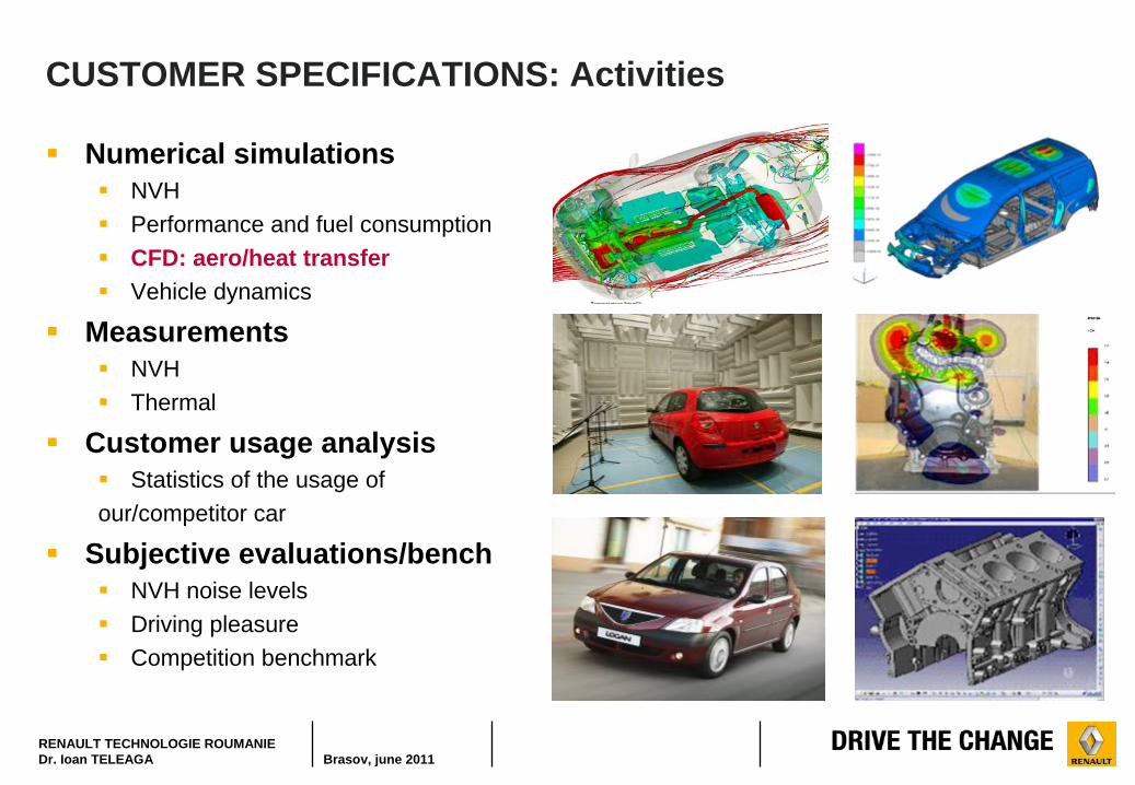
CUSTOMER SPECIFICATIONS: Activities
Numerical simulations
NVH
Performance and fuel consumption
CFD: aero/heat transfer
Vehicle dynamics
Measurements
NVH
Thermal
Customer usage analysis
Statistics of the usage of our/competitor car
Subjective evaluations/bench
NVH noise levels
Driving pleasure
Competition benchmark
RENAULT TECHNOLOGIE ROUMANIEDr. Ioan TELEAGA Brasov, june 2011
02 FROM THEORY TO NUMERICS
RENAULT TECHNOLOGIE ROUMANIEDr. Ioan TELEAGA Brasov, june 2011
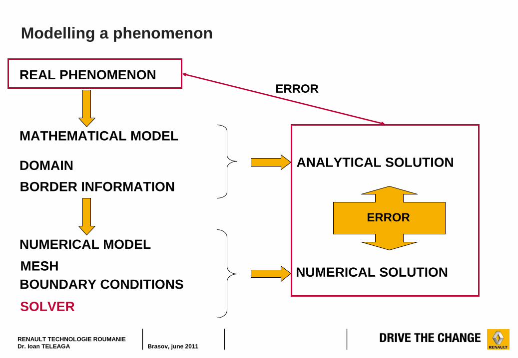
Modelling a phenomenon
REAL PHENOMENON
MATHEMATICAL MODEL
NUMERICAL MODEL
ANALYTICAL SOLUTION
NUMERICAL SOLUTION
DOMAIN
MESH
BORDER INFORMATION
BOUNDARY CONDITIONS
ERROR
SOLVER
ERROR
RENAULT TECHNOLOGIE ROUMANIEDr. Ioan TELEAGA Brasov, june 2011
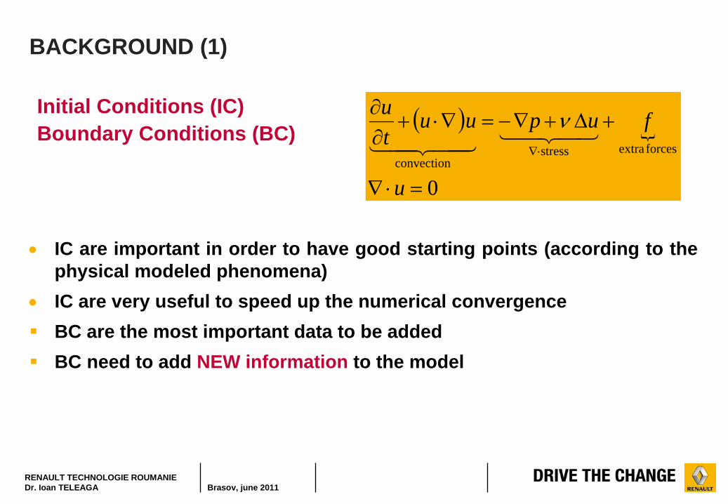
BACKGROUND (1)
IC are important in order to have good starting points (according to the physical modeled phenomena)
IC are very useful to speed up the numerical convergence
BC are the most important data to be added
BC need to add NEW information to the model
0
forcesextrastressconvection
u
fupuutu
Initial Conditions (IC)Boundary Conditions (BC)
RENAULT TECHNOLOGIE ROUMANIEDr. Ioan TELEAGA Brasov, june 2011
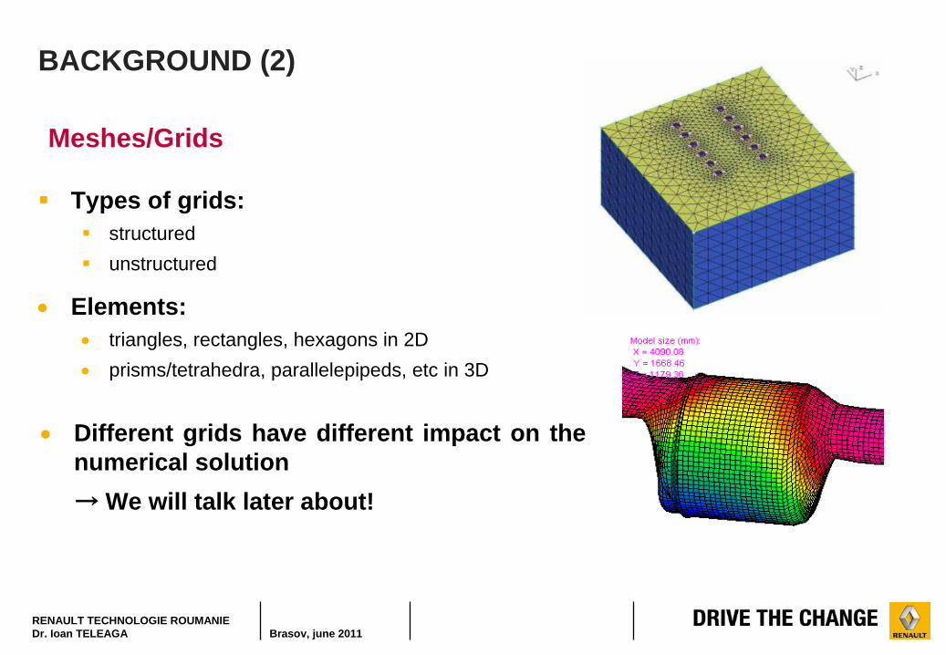
BACKGROUND (2)
Types of grids:
structured
unstructured
Elements:
triangles, rectangles, hexagons in 2D
prisms/tetrahedra, parallelepipeds, etc in 3D
Meshes/Grids
Different grids have different impact on the numerical solution → We will talk later about!
RENAULT TECHNOLOGIE ROUMANIEDr. Ioan TELEAGA Brasov, june 2011
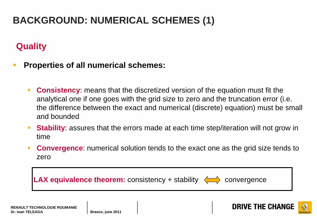
BACKGROUND: NUMERICAL SCHEMES (1)
Properties of all numerical schemes:
Consistency: means that the discretized version of the equation must fit the analytical one if one goes with the grid size to zero and the truncation error (i.e. the difference between the exact and numerical (discrete) equation) must be small and bounded
Stability: assures that the errors made at each time step/iteration will not grow in time
Convergence: numerical solution tends to the exact one as the grid size tends to zero
RENAULT TECHNOLOGIE ROUMANIEDr. Ioan TELEAGA Brasov, june 2011
BACKGROUND: NUMERICAL SCHEMES (2)
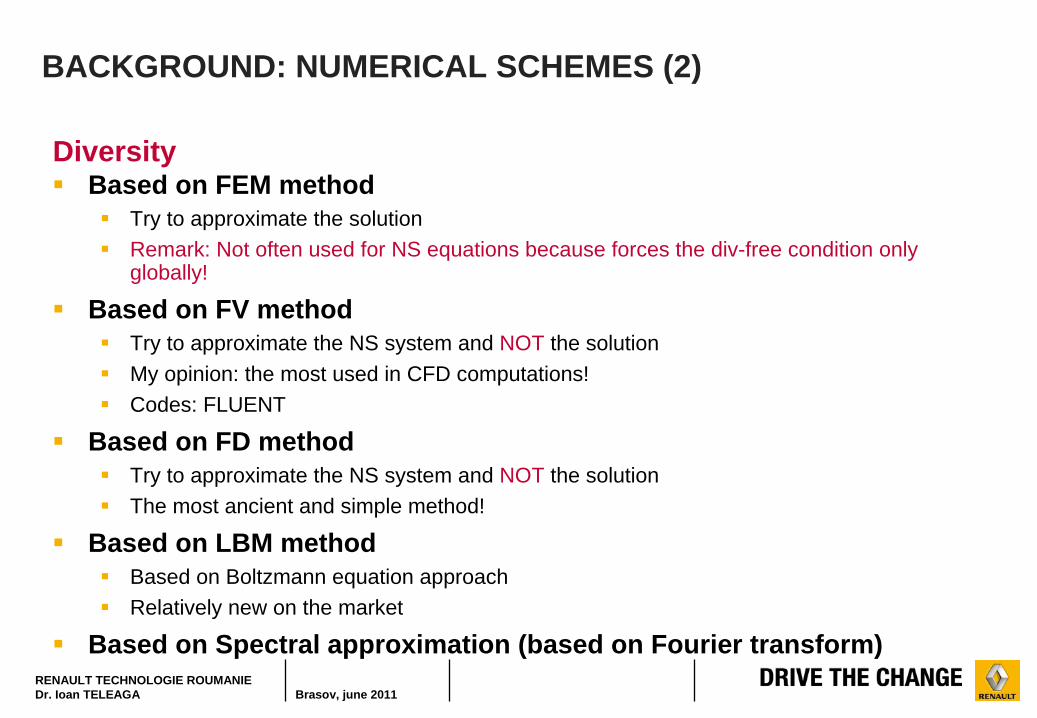
Based on FEM method
Try to approximate the solution
Remark: Not often used for NS equations because forces the div-free condition only globally!
Based on FV method
Try to approximate the NS system and NOT the solution
My opinion: the most used in CFD computations!
Codes: FLUENT
Based on FD method
Try to approximate the NS system and NOT the solution
The most ancient and simple method!
Based on LBM method
Based on Boltzmann equation approach
Relatively new on the market
Based on Spectral approximation (based on Fourier transform)
Diversity
RENAULT TECHNOLOGIE ROUMANIEDr. Ioan TELEAGA Brasov, june 2011
NUMERICAL SCHEMES (2)
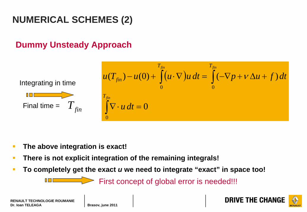
The above integration is exact!
There is not explicit integration of the remaining integrals!
To completely get the exact u we need to integrate “exact” in space too!
fin
finfin
T
TT
fin
dtu
dtfupdtuuuTu
0
00
0
)()0()(
Dummy Unsteady Approach
Final time = finT
Integrating in time
First concept of global error is needed!!!
RENAULT TECHNOLOGIE ROUMANIEDr. Ioan TELEAGA Brasov, june 2011
NUMERICAL SCHEMES (3)
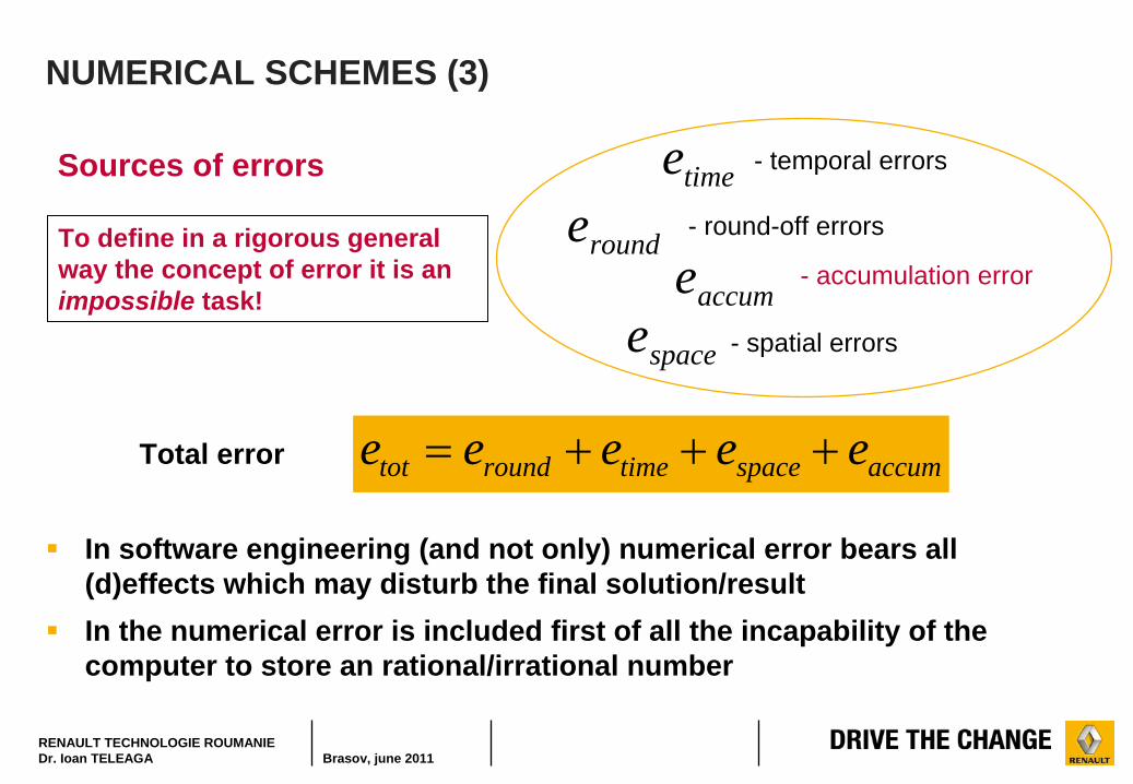
In software engineering (and not only) numerical error bears all (d)effects which may disturb the final solution/result
In the numerical error is included first of all the incapability of the computer to store an rational/irrational number
Sources of errors
accumspacetimeroundtot eeeee Total error
rounde - round-off errors
spacee - spatial errors
accume - accumulation error
timee - temporal errors
To define in a rigorous general way the concept of error it is an impossible task!
RENAULT TECHNOLOGIE ROUMANIEDr. Ioan TELEAGA Brasov, june 2011
SPATIAL ERRORS
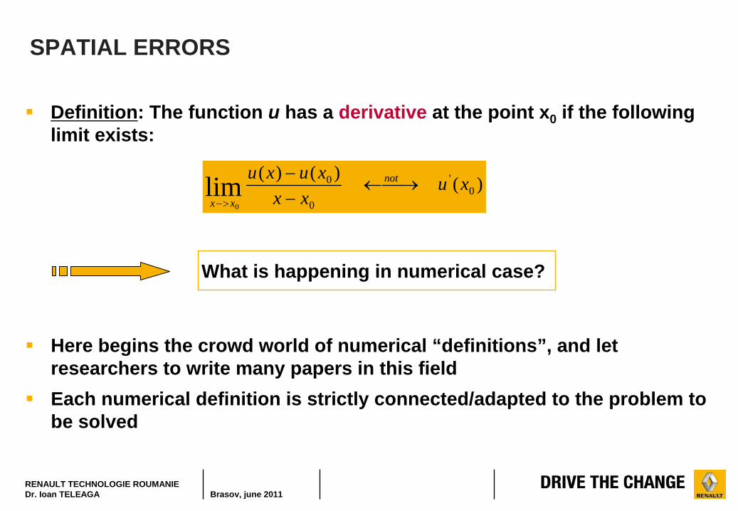
Definition: The function u has a derivative at the point x0 if the following limit exists:
)()()(0
'
0
0lim0
xuxx
xuxu not
xx
What is happening in numerical case?
Here begins the crowd world of numerical “definitions”, and let researchers to write many papers in this field
Each numerical definition is strictly connected/adapted to the problem to be solved
RENAULT TECHNOLOGIE ROUMANIEDr. Ioan TELEAGA Brasov, june 2011
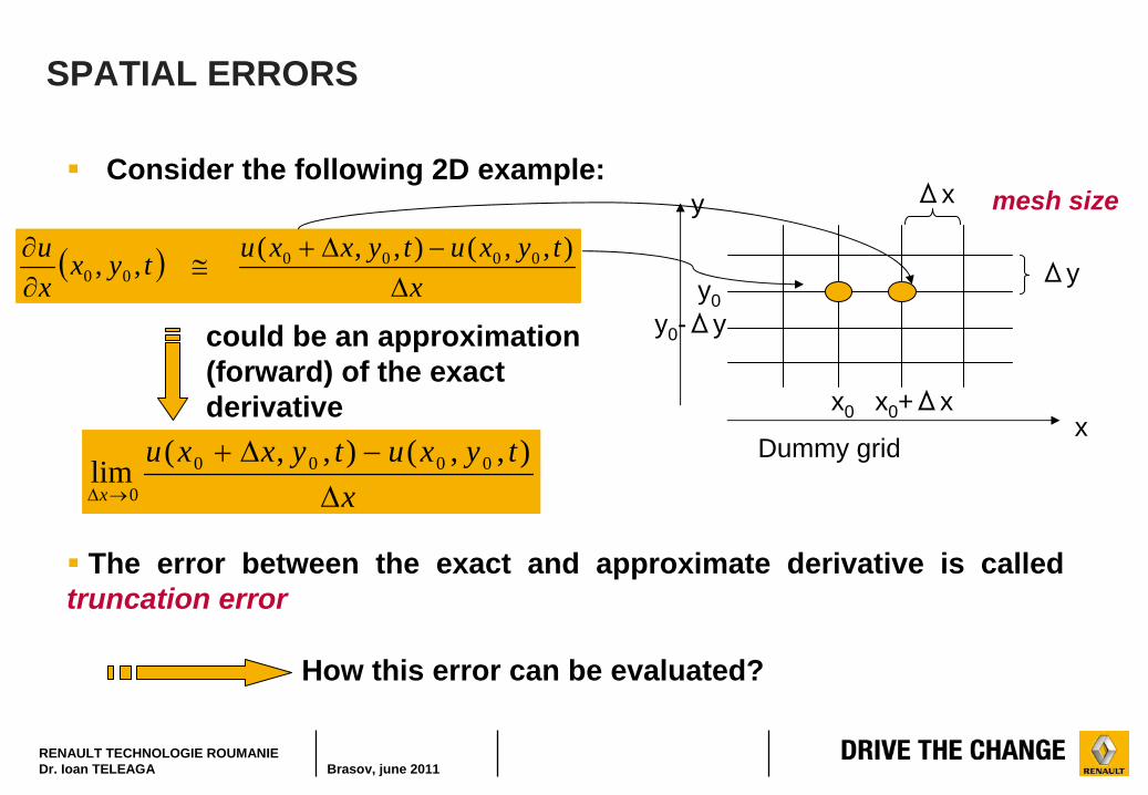
SPATIAL ERRORS
Consider the following 2D example:
x
tyxutyxxutyxxu
),,(),,(,, 0000
00
could be an approximation (forward) of the exact derivative
xtyxutyxxu
x
),,(),,(lim 0000
0
The error between the exact and approximate derivative is called truncation error
How this error can be evaluated?
mesh size
x
y
x0
y0
x0 +Δx
y0 -Δy
Δx
Δy
Dummy grid
RENAULT TECHNOLOGIE ROUMANIEDr. Ioan TELEAGA Brasov, june 2011
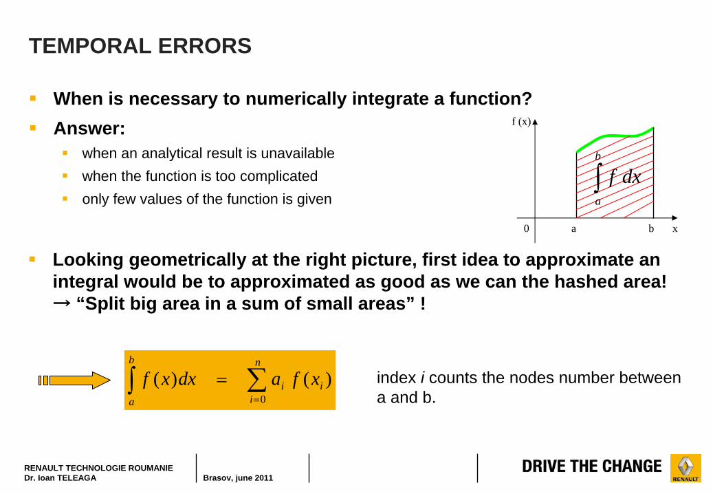
TEMPORAL ERRORS
When is necessary to numerically integrate a function?
Answer:
when an analytical result is unavailable
when the function is too complicated
only few values of the function is given
0 x
f (x)
a b
b
a
dxf
Looking geometrically at the right picture, first idea to approximate an integral would be to approximated as good as we can the hashed area! → “Split big area in a sum of small areas” !
n
iii
b
a
xfadxxf0
)()( index i counts the nodes number between a and b.
RENAULT TECHNOLOGIE ROUMANIEDr. Ioan TELEAGA Brasov, june 2011
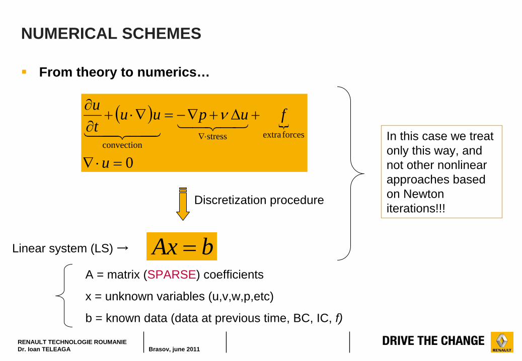
NUMERICAL SCHEMES
From theory to numerics…
0
forcesextrastressconvection
u
fupuutu
bAx
Discretization procedure
Linear system (LS) →
In this case we treat only this way, and not other nonlinear approaches based on Newton iterations!!!
A = matrix (SPARSE) coefficients
x = unknown variables (u,v,w,p,etc)
b = known data (data at previous time, BC, IC, f)
RENAULT TECHNOLOGIE ROUMANIEDr. Ioan TELEAGA Brasov, june 2011
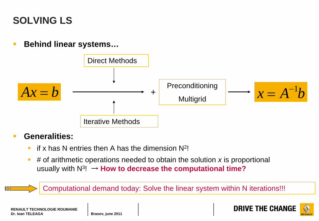
SOLVING LS
Behind linear systems…
bAx
Direct Methods
Iterative Methods
bAx 1+Preconditioning
Multigrid
Generalities:
if x has N entries then A has the dimension N2!
# of arithmetic operations needed to obtain the solution x is proportional usually with N3! → How to decrease the computational time?
Computational demand today: Solve the linear system within N iterations!!!
RENAULT TECHNOLOGIE ROUMANIEDr. Ioan TELEAGA Brasov, june 2011
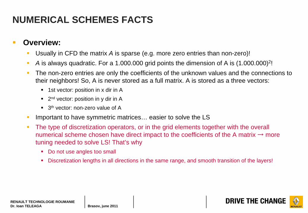
NUMERICAL SCHEMES FACTS
Overview:
Usually in CFD the matrix A is sparse (e.g. more zero entries than non-zero)!
A is always quadratic. For a 1.000.000 grid points the dimension of A is (1.000.000)2!
The non-zero entries are only the coefficients of the unknown values and the connections to their neighbors! So, A is never stored as a full matrix. A is stored as a three vectors:
1st vector: position in x dir in A
2nd vector: position in y dir in A
3th vector: non-zero value of A
Important to have symmetric matrices… easier to solve the LS
The type of discretization operators, or in the grid elements together with the overall numerical scheme chosen have direct impact to the coefficients of the A matrix → more tuning needed to solve LS! That’s why
Do not use angles too small
Discretization lengths in all directions in the same range, and smooth transition of the layers!
RENAULT TECHNOLOGIE ROUMANIEDr. Ioan TELEAGA Brasov, june 2011
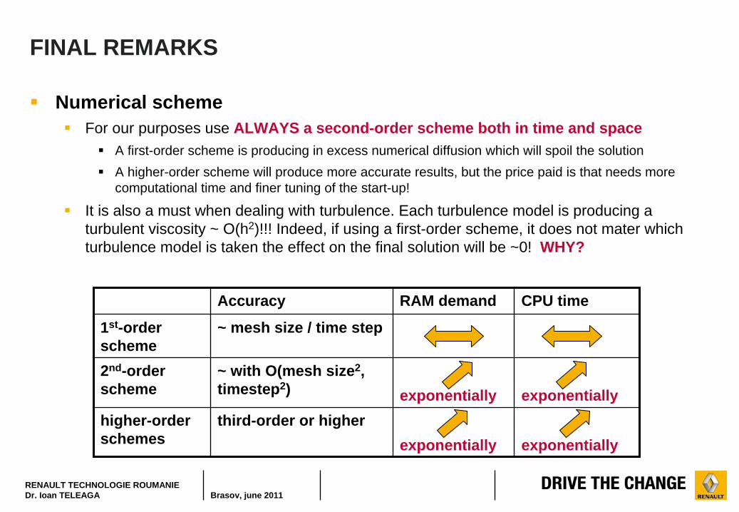
FINAL REMARKS
Numerical scheme
For our purposes use ALWAYS a second-order scheme both in time and space
A first-order scheme is producing in excess numerical diffusion which will spoil the solution
A higher-order scheme will produce more accurate results, but the price paid is that needs more computational time and finer tuning of the start-up!
It is also a must when dealing with turbulence. Each turbulence model is producing a turbulent viscosity ~ O(h2)!!! Indeed, if using a first-order scheme, it does not mater which turbulence model is taken the effect on the final solution will be ~0! WHY?
Accuracy RAM demand CPU time
1st-order scheme
~ mesh size / time step
2nd-order scheme
~ with O(mesh size2, timestep2) exponentially exponentially
higher-order schemes
third-order or higherexponentially exponentially
RENAULT TECHNOLOGIE ROUMANIEDr. Ioan TELEAGA Brasov, june 2011
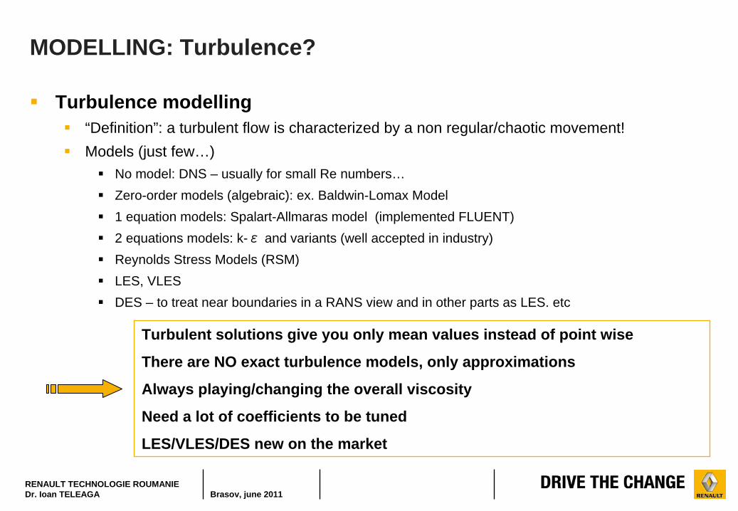
MODELLING: Turbulence?
Turbulence modelling
“Definition”: a turbulent flow is characterized by a non regular/chaotic movement!
Models (just few…)
No model: DNS – usually for small Re numbers…
Zero-order models (algebraic): ex. Baldwin-Lomax Model
1 equation models: Spalart-Allmaras model (implemented FLUENT)
2 equations models: k-ε and variants (well accepted in industry)
Reynolds Stress Models (RSM)
LES, VLES
DES – to treat near boundaries in a RANS view and in other parts as LES. etc
Turbulent solutions give you only mean values instead of point wise
There are NO exact turbulence models, only approximations
Always playing/changing the overall viscosity
Need a lot of coefficients to be tuned
LES/VLES/DES new on the market
RENAULT TECHNOLOGIE ROUMANIEDr. Ioan TELEAGA Brasov, june 2011
03 AERODYNAMICS
RENAULT TECHNOLOGIE ROUMANIEDr. Ioan TELEAGA Brasov, june 2011
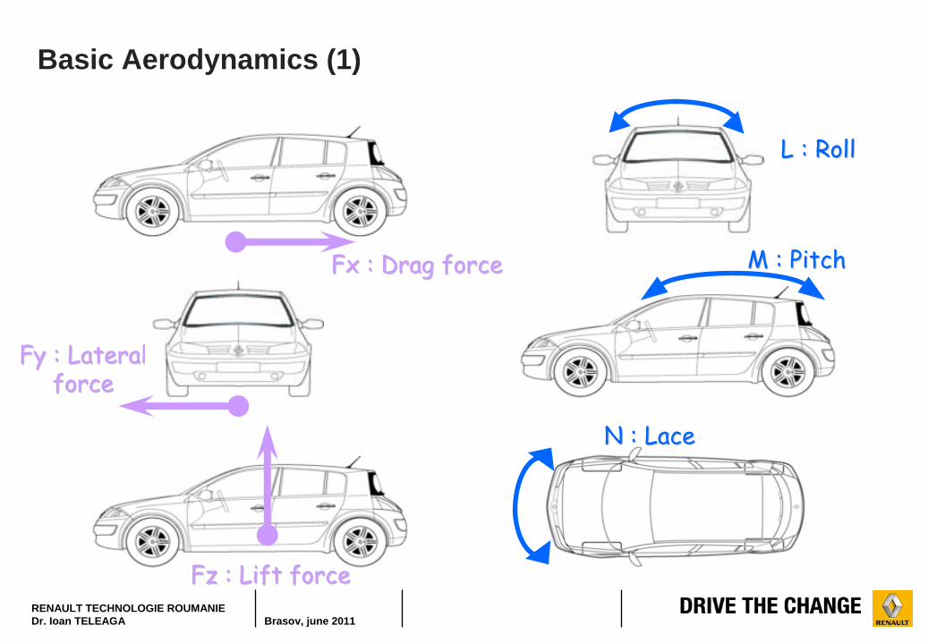
Basic Aerodynamics (1)
Fx : Drag forceFx : Drag force
Fy : Lateral Fy : Lateral forceforce
Fz : Lift forceFz : Lift force
L : RollL : Roll
M : PitchM : Pitch
N : LaceN : Lace
RENAULT TECHNOLOGIE ROUMANIEDr. Ioan TELEAGA Brasov, june 2011
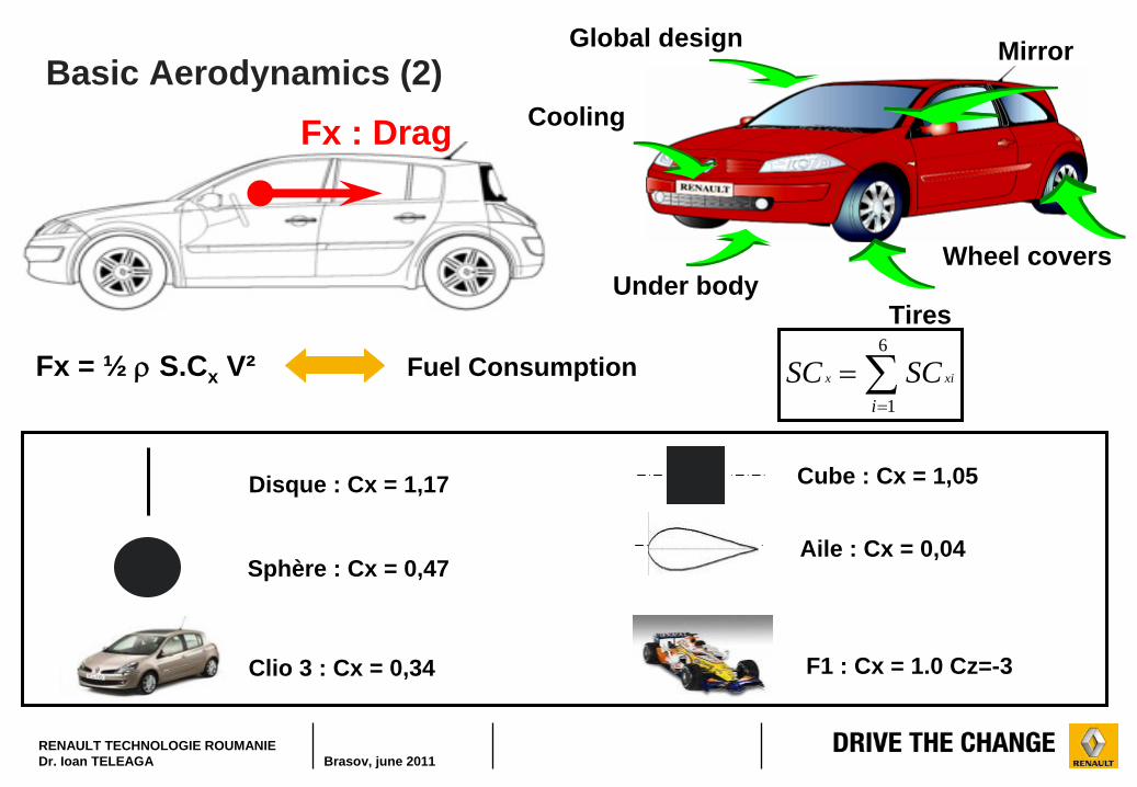
Fx = ½
S.Cx V² Fuel Consumption
Fx : Drag
Sphère : Cx = 0,47
Disque : Cx = 1,17 Cube : Cx = 1,05
Aile : Cx = 0,04
Clio 3 : Cx = 0,34 F1 : Cx = 1.0 Cz=-3
Cooling
Tires
Mirror
Under bodyWheel covers
Global design
6
1ixix SCSC
Basic Aerodynamics (2)
RENAULT TECHNOLOGIE ROUMANIEDr. Ioan TELEAGA Brasov, june 2011
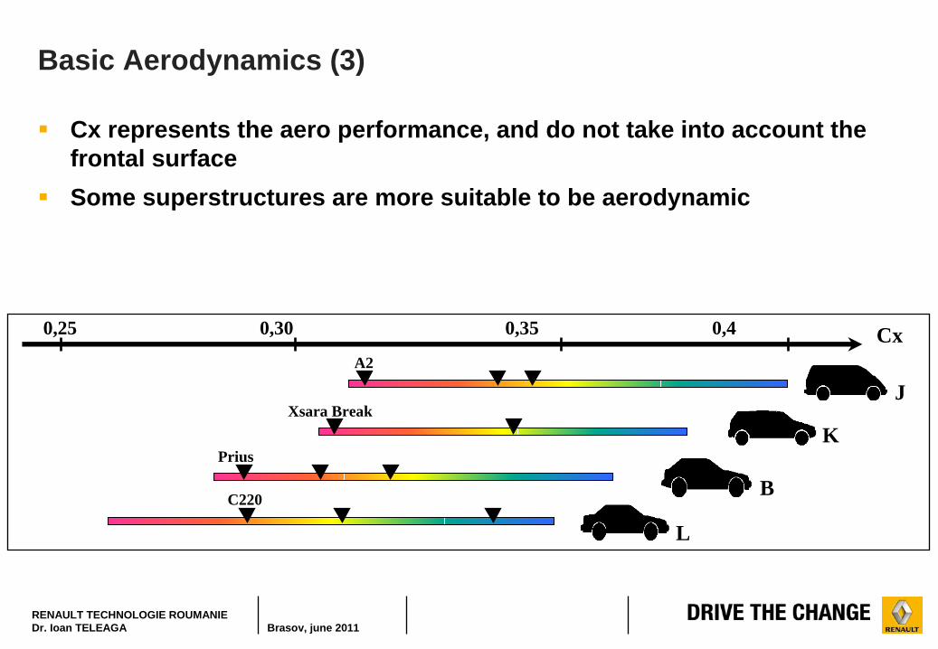
Basic Aerodynamics (3)
Cx0,25 0,30 0,35 0,4
A2
JXsara Break
K
BPrius
C220
L
Cx represents the aero performance, and do not take into account the frontal surface
Some superstructures are more suitable to be aerodynamic
RENAULT TECHNOLOGIE ROUMANIEDr. Ioan TELEAGA Brasov, june 2011
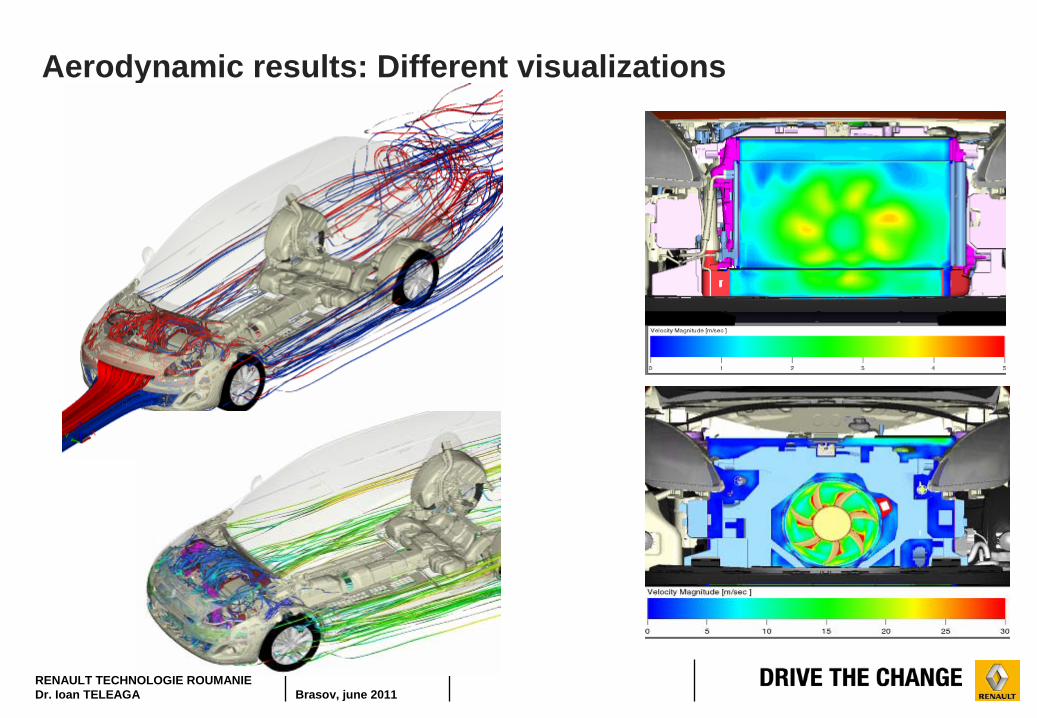
Aerodynamic results: Different visualizations
RENAULT TECHNOLOGIE ROUMANIEDr. Ioan TELEAGA Brasov, june 2011
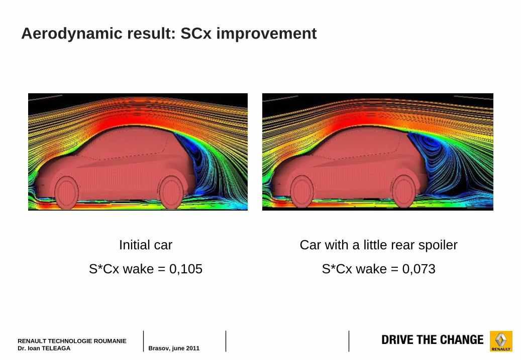
Car with a little rear spoiler
S*Cx wake = 0,073
Initial car
S*Cx wake = 0,105
Aerodynamic result: SCx improvement
RENAULT TECHNOLOGIE ROUMANIEDr. Ioan TELEAGA Brasov, june 2011
04 HEAT TRANSFER
RENAULT TECHNOLOGIE ROUMANIEDr. Ioan TELEAGA Brasov, june 2011
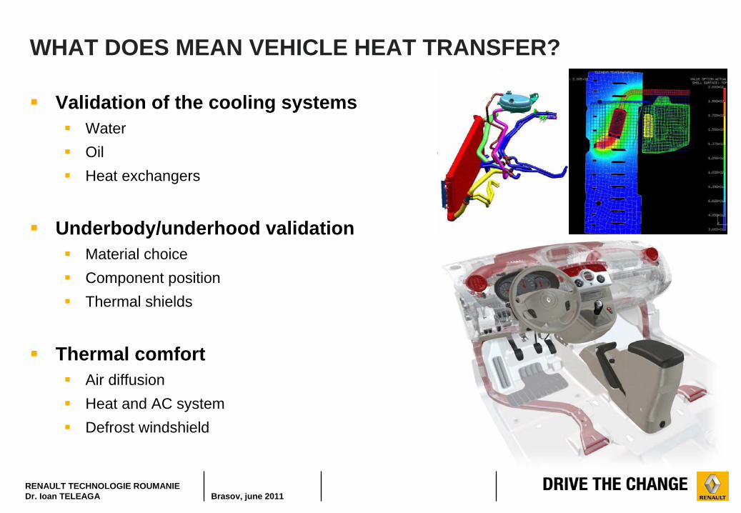
WHAT DOES MEAN VEHICLE HEAT TRANSFER?
Validation of the cooling systems
Water
Oil
Heat exchangers
Underbody/underhood validation
Material choice
Component position
Thermal shields
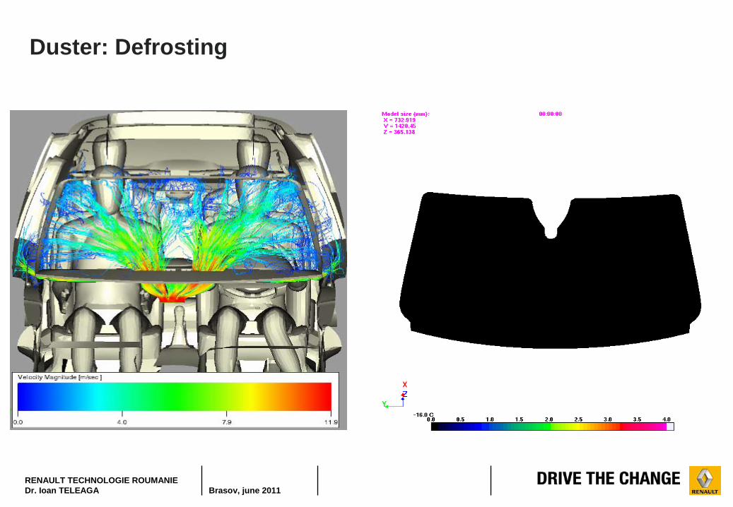
Thermal comfort
Air diffusion
Heat and AC system
Defrost windshield
RENAULT TECHNOLOGIE ROUMANIEDr. Ioan TELEAGA Brasov, june 2011
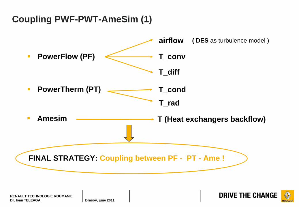
Coupling PWF-PWT-AmeSim (1)
PowerFlow (PF)
FINAL STRATEGY: Coupling between PF - PT - Ame !
airflow
T_conv
T_diff
T_cond
T_rad
( DES as turbulence model )
T (Heat exchangers backflow)
Amesim
PowerTherm (PT)
RENAULT TECHNOLOGIE ROUMANIEDr. Ioan TELEAGA Brasov, june 2011
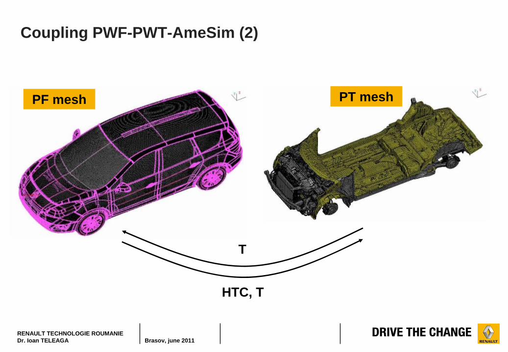
Coupling PWF-PWT-AmeSim (2)
T
HTC, T
PF mesh PT mesh
RENAULT TECHNOLOGIE ROUMANIEDr. Ioan TELEAGA Brasov, june 2011
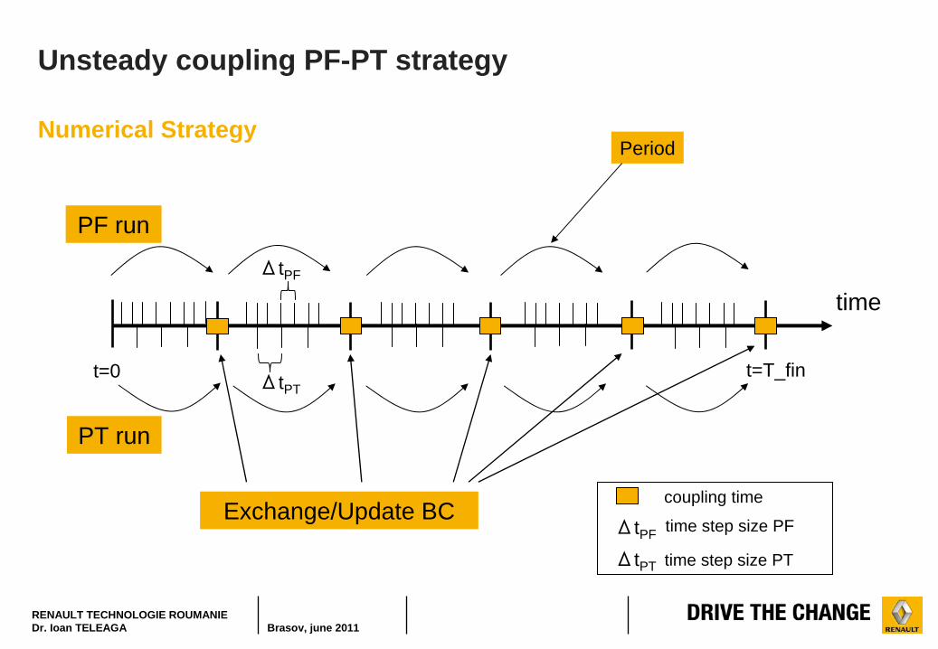
Unsteady coupling PF-PT strategy
Numerical Strategy
t=0 t=T_fin
time
coupling time
Period
PF run
PT run
ΔtPT
ΔtPF
ΔtPF
ΔtPT
time step size PF
time step size PT
Exchange/Update BC
RENAULT TECHNOLOGIE ROUMANIEDr. Ioan TELEAGA Brasov, june 2011
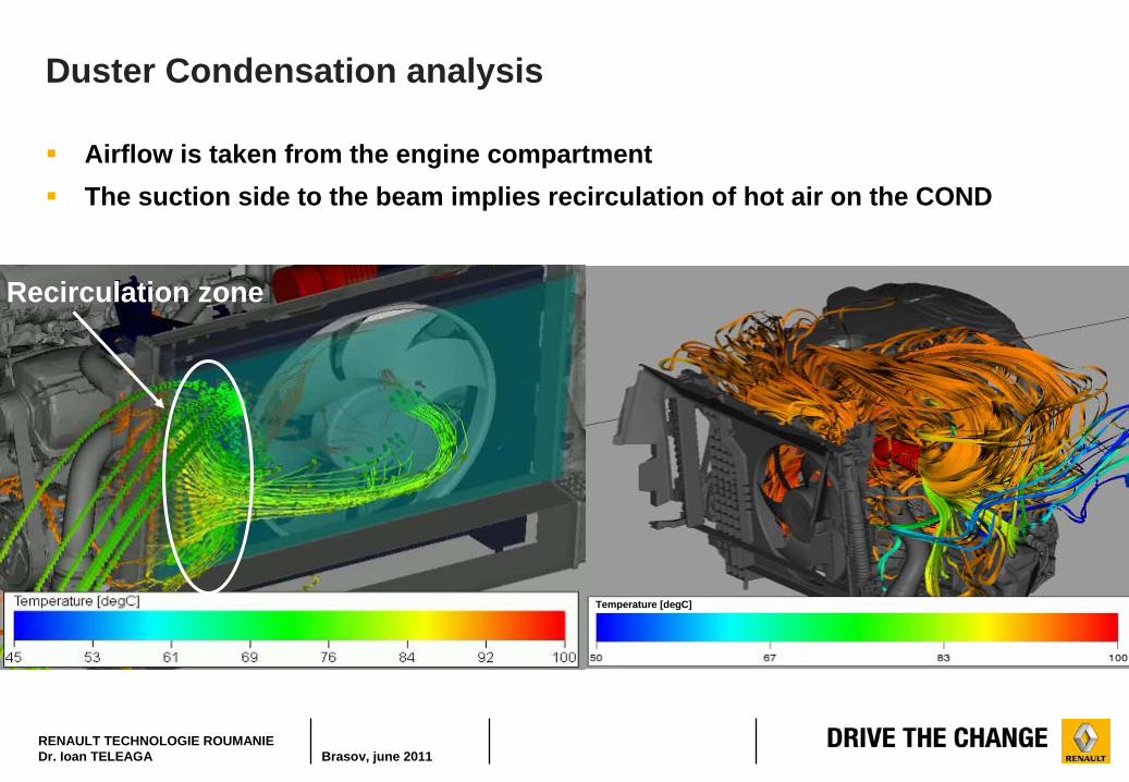
Duster Condensation analysis
Airflow is taken from the engine compartment
The suction side to the beam implies recirculation of hot air on the COND
Temperature [degC]
Recirculation zonesRecirculation zone
RENAULT TECHNOLOGIE ROUMANIEDr. Ioan TELEAGA Brasov, june 2011
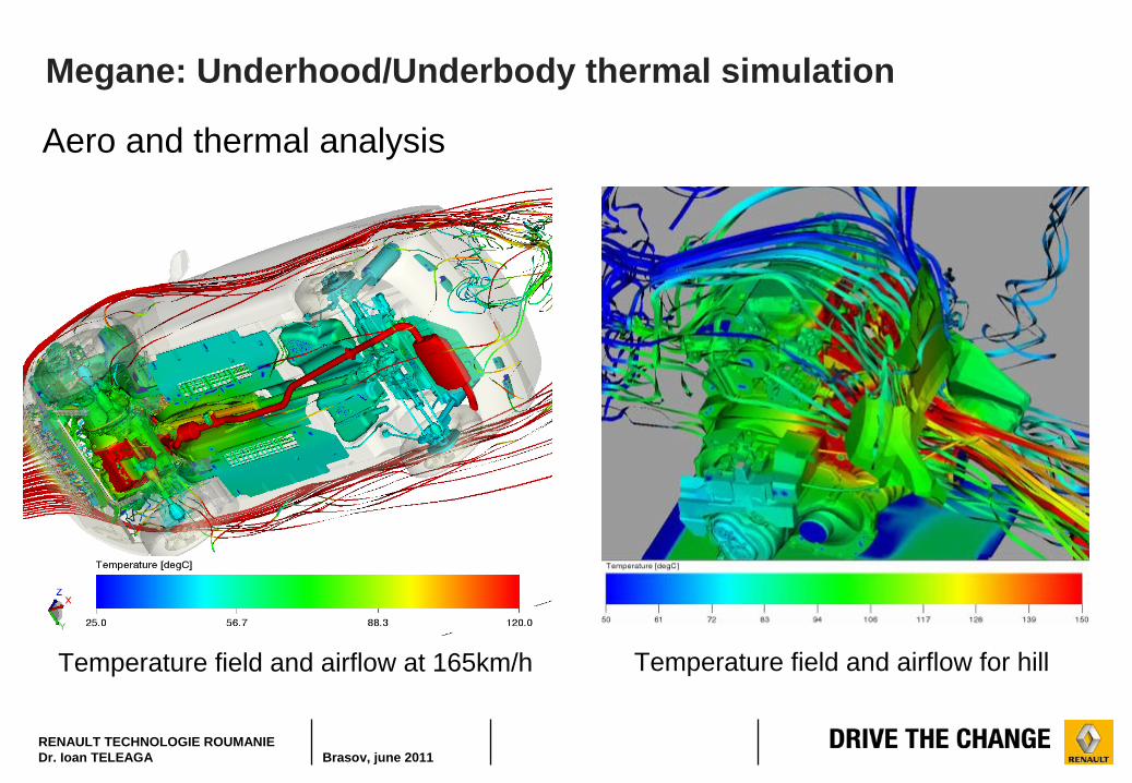
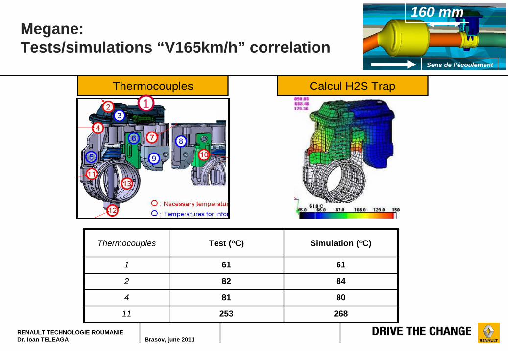
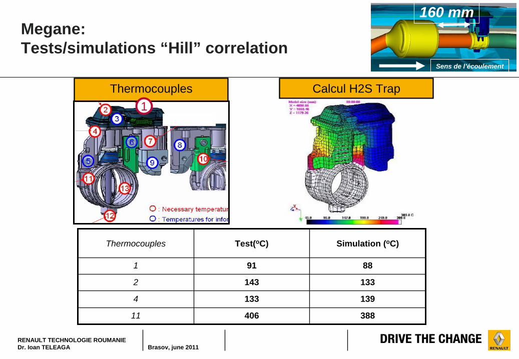
Megane: Underhood/Underbody thermal simulation
Temperature field and airflow for hillTemperature field and airflow at 165km/h
Aero and thermal analysis
RENAULT TECHNOLOGIE ROUMANIEDr. Ioan TELEAGA Brasov, june 2011
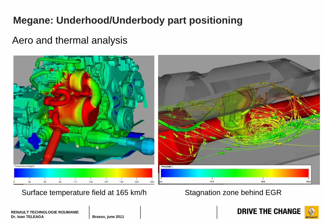
Megane: Underhood/Underbody part positioning
Surface temperature field at 165 km/h Stagnation zone behind EGR
Aero and thermal analysis
RENAULT TECHNOLOGIE ROUMANIEDr. Ioan TELEAGA Brasov, june 2011
RENAULT TECHNOLOGIE ROUMANIEDr. Ioan TELEAGA Brasov, june 2011
Duster: Defrosting
RENAULT TECHNOLOGIE ROUMANIEDr. Ioan TELEAGA Brasov, june 2011
Conclusions
Scientific computation is used with success within Renault
Nowadays experiments and theory are supplemented in many cases by numerical computation that is an equally important component
Within scientific computing one can treat more complex and less simplified problems through massive amounts of numerical calculations and thanks to the increased computer facilities in short time
RENAULT TECHNOLOGIE ROUMANIEDr. Ioan TELEAGA Brasov, june 2011 39