Institutul Naţional Societatea Română de Statistică de Statistică ROMANIAN STATISTICAL REVIEW - SUPPLEMENT - INTERNATIONAL SYMPOSIUM “Romania and the Economic-Financial Crisis. Methods and Models for Macroeconomic Analysis” 2013
Transcript
Institutul Naţional Societatea Română de Statistică de Statistică
ROMANIAN STATISTICAL REVIEW - SUPPLEMENT -
INTERNATIONAL SYMPOSIUM
“Romania and the Economic-Financial
Crisis. Methods and Models for Macroeconomic Analysis”
2013
Autorii poartă întreaga răspundere pentru conţinutul materialelor publicate, revista şi Societatea Română
de Statistică fiind exonerate de orice răspundere.
ISSN 1018-046x
“ARTIFEX” UNIVERSITY OF BUCHAREST
INTERNATIONAL SYMPOSIUM
“Romania and the Economic-Financial Crisis. Methods and Models for Macroeconomic Analysis”
MAY 23-24, 2013
Bucharest, Romania
ACADEMY OF ECONOMIC STUDIES OF MOLDAVIA
MEDIA PARTNER The Romanian Statistical Review
POLITECHNIC UNIVERSITY OF CZESTOCHOWA,
POLAND
VALACHIA UNIVERSITY, TARGOVISTE
ACADEMY OF ECONOMIC STUDIES, BUCHAREST
DEPARTMENT OF STATISTICS AND ECONOMETRICS
TECHNICAL UNIVERSITY OF KOSICE - SLOVAKIA
PRESIDENTS OF HONOUR Prof. Dan Cruceru, PhD – President of the”Artifex” University of Bucharest Prof. Constantin Anghelache, PhD – President of the Senate, ”Artifex” University of Bucharest Prof. Mircea Udrescu, PhD – Rector, ”Artifex” University of Bucharest Prof. Grigore Belostecinic, PhD – Rector of the Academy of Economic Studies, the Republic of Moldavia Prof. Ioan Lucian Albu, PhD, Member of the Romanian Academy Prof. Vergil Voineagu, PhD – Academy of Economic Studies, Bucharest ORGANIZING COMMITTEE Prof. Mircea Udrescu, PhD - ”Artifex” University of Bucharest Assoc. prof. Elena Bugudui, PhD - ”Artifex” University of Bucharest Assoc. prof. Aurelian Diaconu, PhD - ”Artifex” University of Bucharest Assoc. prof. Sorin Gabriel Gresoi, PhD - ”Artifex” University of Bucharest Assoc. prof. Emanuela Ionescu, PhD - ”Artifex” University of Bucharest Assoc. prof. Dan Năstase, PhD - ”Artifex” University of Bucharest Assoc. prof. Anca Mihaela Teau, PhD - ”Artifex” University of Bucharest Assoc. prof. Dragoş Rădulescu, PhD – “Dimitrie Cantemir” Christian University of Bucharest Assoc. prof. Luminiţa Dragne, PhD – “Dimitrie Cantemir” Christian University of Bucharest Assoc. prof. Agata Popescu, PhD – “Dimitrie Cantemir” Christian University of Bucharest Assoc. prof. Ancuţa Geanina Opre, PhD – “Dimitrie Cantemir” Christian University of Bucharest Lecturer Andrei Buiga, PhD - ”Artifex” University of Bucharest Lecturer Cătălin Deatcu, PhD- ”Artifex” University of Bucharest Lecturer Cristina Elena Protopopescu, PhD - ”Artifex” University of Bucharest Lecturer Mădălina Anghel, PhD Student - ”Artifex” University of Bucharest Assistant Andreea Gabriela Baltac, PhD Student”Artifex” University of Bucharest Adina Mihaela Dinu, PhD Student - Academy of Economic Studies, Bucharest Assistant Ligia Prodan, PhD Student - Academy of Economic Studies, Bucharest SCIENTIFIC COMMITTEE Prof. Dumitru Moldovan, PhD,- Member of the Academy of the Republic of Moldavia Prof. Maria Nowicka-Skowron, PhD, Politechnic University of Czestochowa, Poland Prof. Janusz Grabara, PhD – Politechnic University of Czestochowa, Poland Prof. Mario Pagliacci, PhD – Università degli Studi di Perugia Prof. Ioan Partachi, PhD – Academy of Economic Studies, the Republic of Moldavia Assoc. prof. Oleg Verejan, PhD – Academy of Economic Studies, the Republic of Moldavia Prof. Josef Novak-Marcincin, PhD – Technical University of Kosice, Slovakia Prof. Vladimir Modrak, PhD – Technical University of Kosice, Slovakia Prof. Vergil Voineagu, PhD – Academy of Economic Studies, Bucharest Prof. Constantin Mitruţ, PhD - President of the Romanian Society of Statistics Prof. Constantin Anghelache, PhD – Vice-president of the Romanian Society of Statistics, Vice-president of the General Association of Economists of Romania Prof. Gabriela Victoria Anghelache, PhD – Academy of Economic Studies, Bucharest Prof. Dan Armeanu, PhD – Academy of Economic Studies, Bucharest Prof. Viorel Lefter, PhD –Academy of Economic Studies, Bucharest Prof. Liviu Begu, PhD – Academy of Economic Studies, Bucharest Prof. Tudorel Andrei, PhD – Academy of Economic Studies, Bucharest Prof. Marin Andreica, PhD – Academy of Economic Studies, Bucharest Prof. Emilia Titan, PhD – Academy of Economic Studies, Bucharest Prof. Ioan Constantin Dima, PhD - “Valachia” University, Targoviste Prof. Ion Stegăroiu, PhD - “Valachia” University, Targoviste Prof. Dorina Tănăsescu, PhD – “Valachia” University, Targoviste Prof. Mariana Man, PhD - University of Petrosani
Prof. Ioan Cosmescu, PhD – “Lucian Blaga” University , Sibiu Prof. Ion Pârgaru, PhD – “Politehnica” University of Bucharest Prof. Gheorghe Lepădatu, PhD – “Dimitrie Cantemir” Christian University of Bucharest Prof. Manoela Popescu, PhD – “Dimitrie Cantemir” Christian University of Bucharest Prof. Viorica Ionaşcu, PhD – “Dimitrie Cantemir” Christian University of Bucharest Assoc. prof. Emilia Gogu, PhD– “Dimitrie Cantemir” Christian University of Bucharest Assoc. prof. Andreea Băltăreţu, PhD – “Dimitrie Cantemir” Christian University of Bucharest Lecturer Bogdan Drăguţ, PhD– “Dimitrie Cantemir” Christian University of Bucharest Prof. Radu Titus Marinescu, PhD – “Artifex” University of Bucharest Assoc. prof. Cristian Barbu, PhD - “Artifex” University of Bucharest Assoc. prof. Anca Sorina Popescu - Cruceru, PhD - “Artifex” University of Bucharest Assoc. prof. Virginia Cucu, PhD - “Artifex” University of Bucharest Assoc. prof. Carmen Valentina Rădulescu, PhD – Academy of Economic Studies of Bucharest Lecturer Ioana Nely Militaru, PhD – Academy of Economic Studies, Bucharest Assoc. prof. Alexandru Manole, PhD – ”Artifex” University of Bucharest
Revista Română de Statistică – Supliment Trim II/2013 7
TABLE OF CONTENTS
Democratic Participation in the Model for Emphasis and Protection of Cooperative Identity and Social-Economic Activity of the Society ............................................................................... 13
Ec. Sevastiţa GRIGORESCU Prof. Dan CRUCERU PhD
Inflation and Unemployment – a Correlative Analysis ......................... 22 Prof. Constantin ANGHELACHE PhD Prof. Vergil VOINEAGU PhD Mihai GHEORGHE PhD Ec. Cristina SACALĂ Ec. Ionuţ NEGOIŢĂ Ec. Alexandru URSACHE
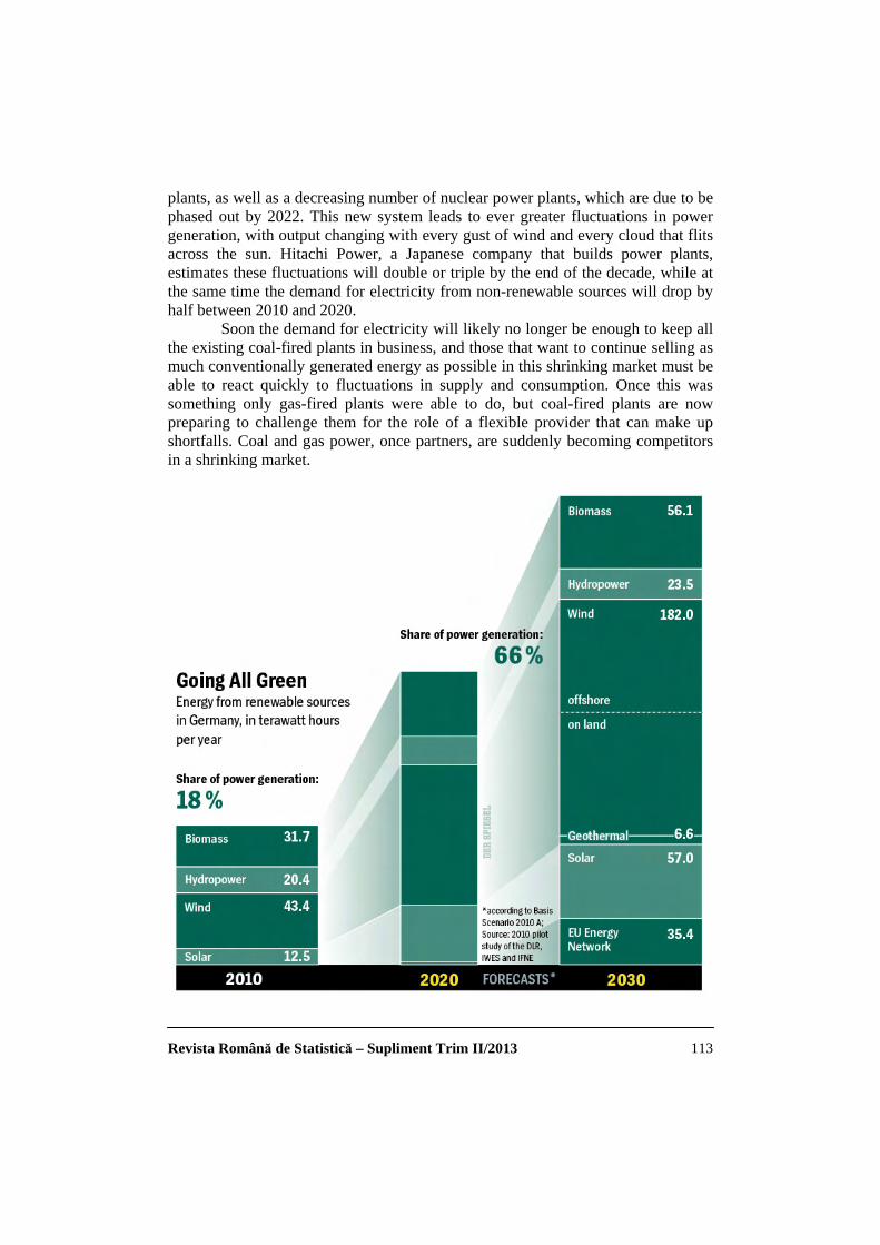
Guaranteeing Energy Supplies ................................................................ 30 Assoc. prof. Alexandru MANOLE PhD Valentin BICHIR PhD Student Alex BODISLAV PhD Student Georgeta BARDAŞU (LIXANDRU) PhD Student Andreea Gabriela BALTAC PhD Student
The Impact of Tax Pressure on Companies’ Performance Case Study: OECD Europe Zone ............................................................ 35
Prof. PhD. Georgeta VINTILĂ Ioana Laura ŢIBULCĂ PhD Candidate
Reforming the Eurozone .......................................................................... 42 Prof. Radu Titus MARINESCU, PhD Prof. Constantin ANGHELACHE, PhD Valentin BICHIR, PhD Student Alex BODISLAV, PhD Student
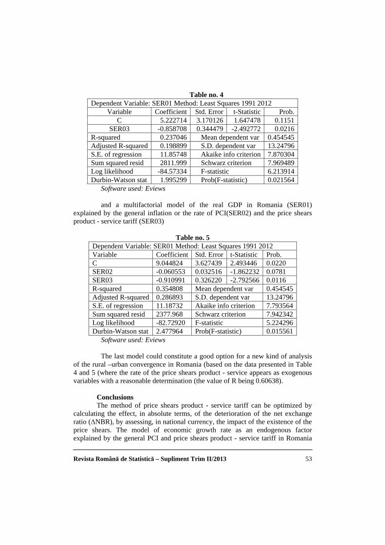
The Relevance of the Rural – Urban Covergence Based on a New Method of Price Shears’ in Romanian Economy ................................... 49
Assoc. prof. Gheorghe SĂVOIU, PhD Prof. Laurenţiu TĂCHICIU, PhD Prof. Vasile DINU, PhD
The Features of the Chronological Series of Statistical Indices............ 55 Prof. Constantin ANGHELACHE PhD Prof. Vergil VOINEAGU PhD Mihai GHEORGHE PhD Ec. Cristina SACALĂ Ec. Ionuţ NEGOIŢĂ Ec. Alexandru URSACHE
Revista Română de Statistică – Supliment Trim II/2013 8
The Relationship between Ecotourism, Responsible Tourism and Cooperative Domain.......................................................................... 62
Prof. Dan CRUCERU PhD Assistant teacher Alina GHEORGHE PhD Student
General Aspects Regarding the Methodology for Prediction Risk .......................................................................................... 66
Prof. Victoria Gabriela ANGHELACHE PhD Ec. Dumitru Cristian OANEA Lecturer Bogdan ZUGRAVU PhD
Attitudes and Behaviors in Negotiation .................................................. 73 Assoc. prof. Cibela NEAGU PhD Assoc. prof. Cezar BRAICU PhD
Theoretical Aspects Regarding the Use of the Multiple Linear Regression Model in Economic Analyses................................................ 78
Prof. Constantin ANGHELACHE PhD Prof. Ioan PARTACHI PhD Adina Mihaela DINU PhD Student Assistant teacher Ligia PRODAN PhD Student Georgeta BARDAŞU (LIXANDRU) PhD Student
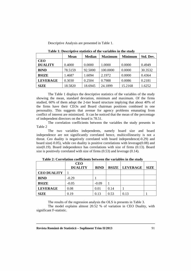
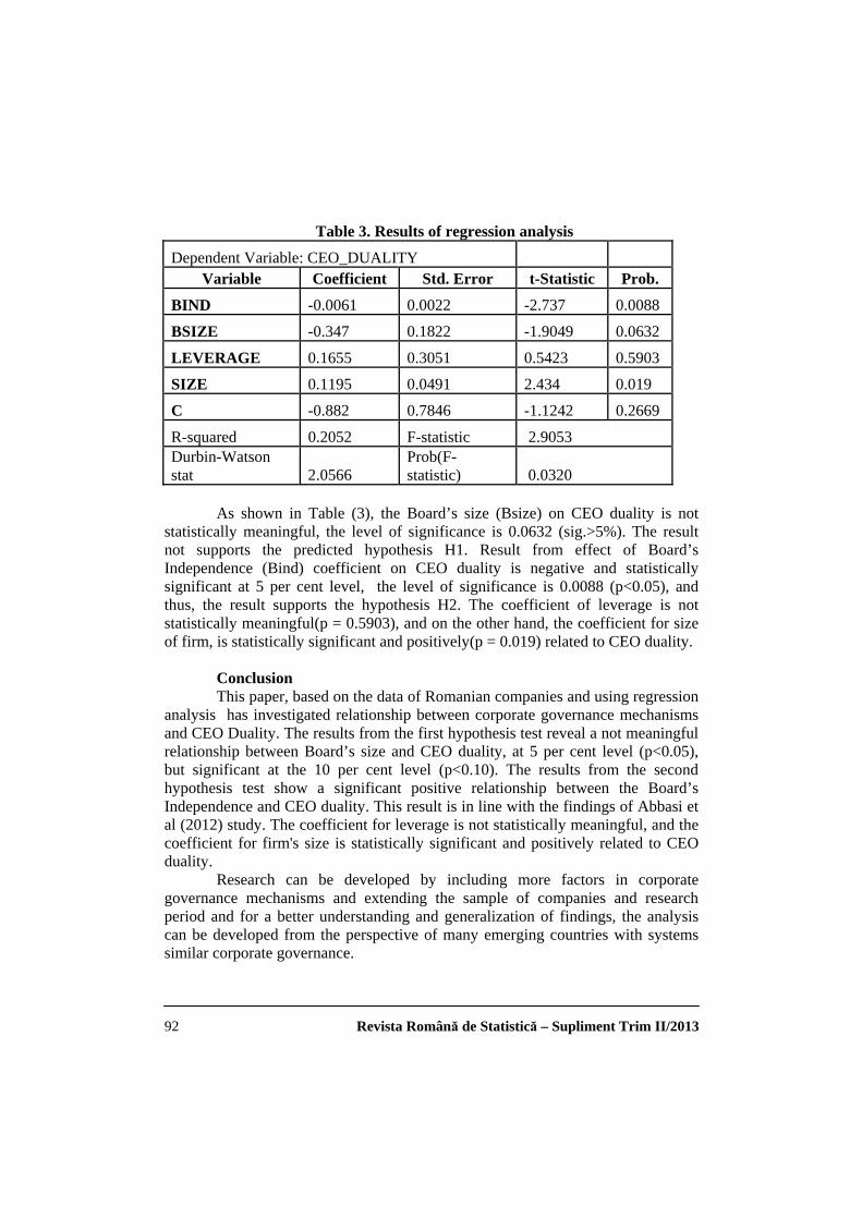
Study on CEO Duality and Corporate Governance of Companies Listed in Bucharest Stock Exchange ....................................................... 88
Prof. Georgeta VINTILǍ Ph D Lecturer Floriniţa DUCA PhD Student
Plan for Internal Audit- Short Considerations ...................................... 94 Assoc. prof. Dan TOGOE PhD
Analytical Methods for the Analysis of Managerial Risk in the Marketing...................................................................................... 101
Svetlana BRADUŢAN PhD Student Energy Management throughout European Union after Fukusima disaster ................................................................................... 106
Prof. Constantin ANGHELACHE, PhD Valentin BICHIR, PhD Student Alex BODISLAV, PhD Student Oleg CARA, PhD
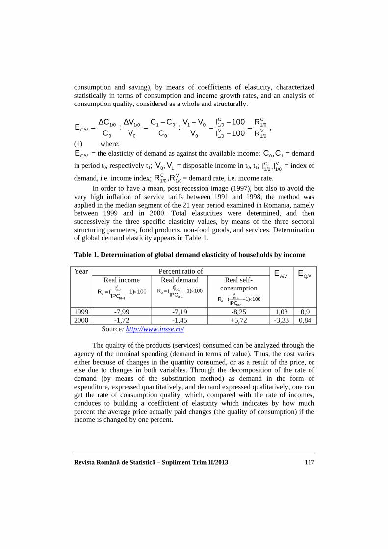
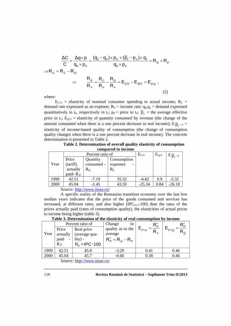
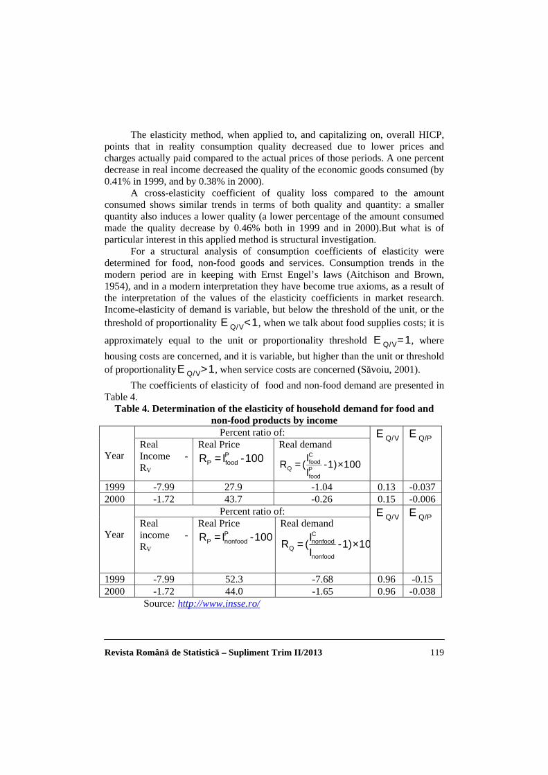
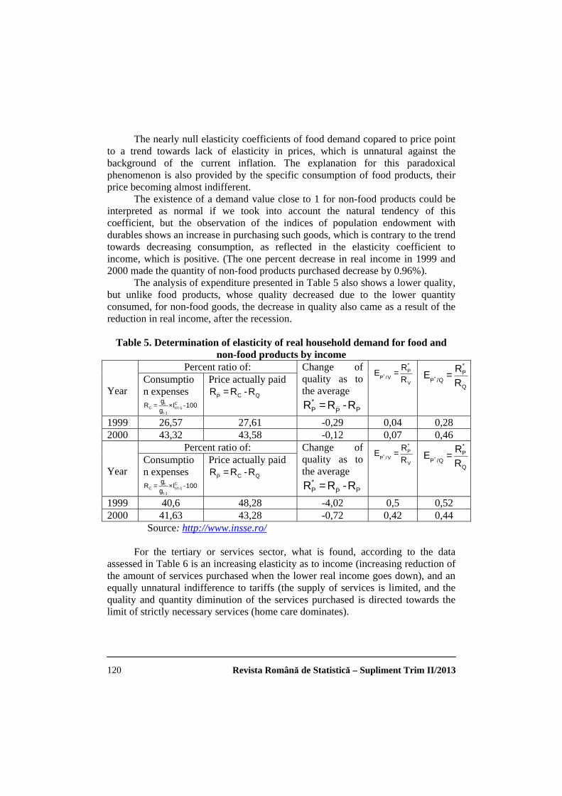
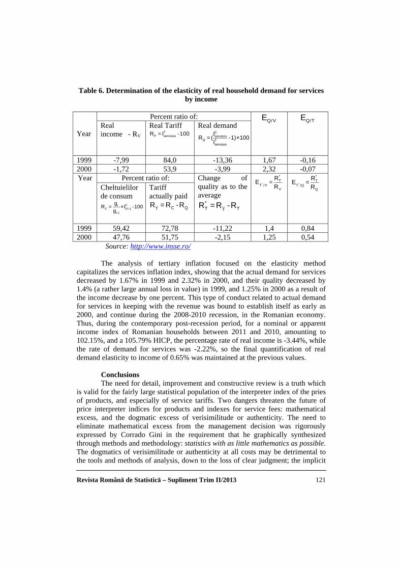
A Statistical Applied Method, Drawing on the Consumer Price Index and its Investigative Qualities............................................ 116
Assoc. prof. Gheorghe SĂVOIU, PhD
Revista Română de Statistică – Supliment Trim II/2013 9
Econometric Model for Risk Forecasting ............................................. 123 Ec. Dumitru Cristian OANEA Prof. Victoria Gabriela ANGHELACHE PhD Lecturer Bogdan ZUGRAVU PhD
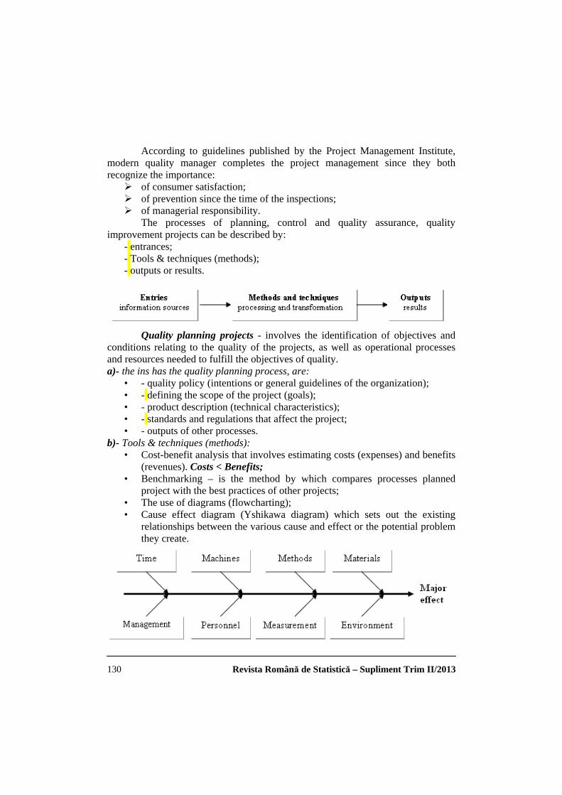
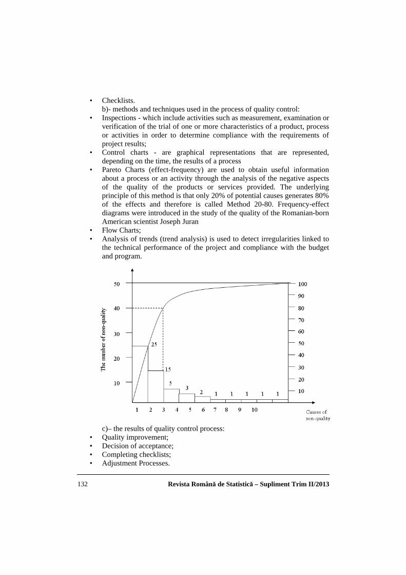
Quality Management of Projects ........................................................... 128 Associate Professor Sorin Gabriel GRESOI PhD Associate Professor Aurelian DIACONU PhD Amelia DIACONU (EFTIMESCU) PhD Student
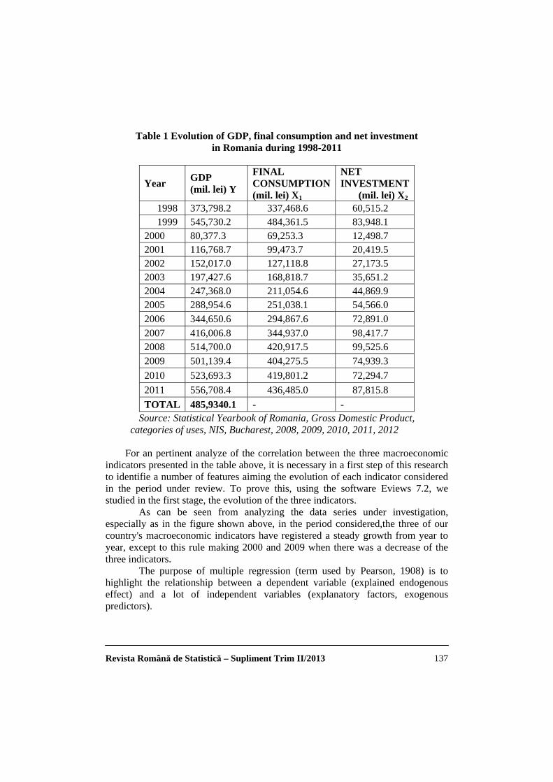
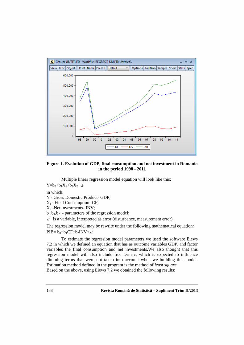
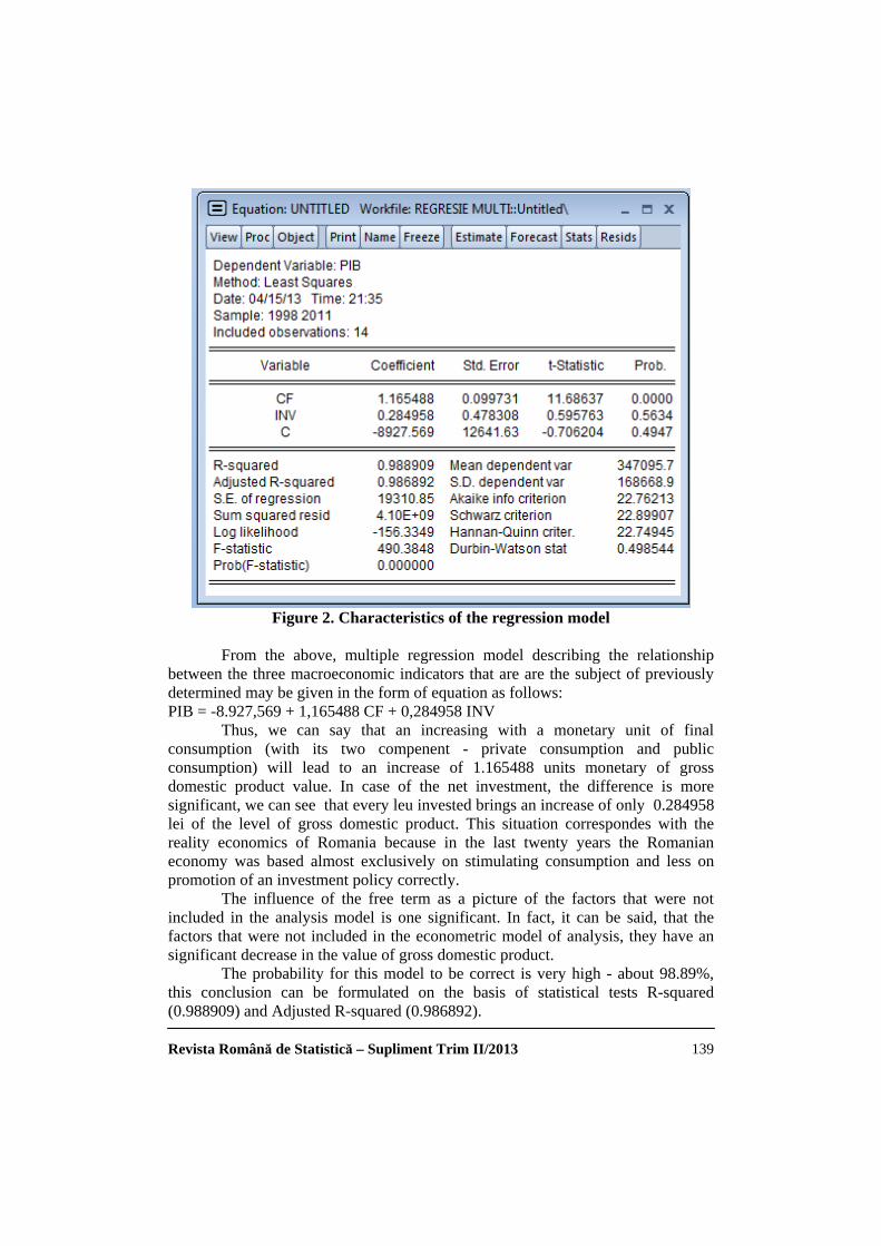
Multiple Regression Used in Macro-economic Analysis .................................................................................................... 134
Prof. Constantin ANGHELACHE PhD Prof. Mario G.R. PAGLIACCI PhD Assoc. prof. Elena BUGUDUI PhD Assistant teacher Ligia PRODAN PhD Student Ec. Bogdan DRAGOMIR
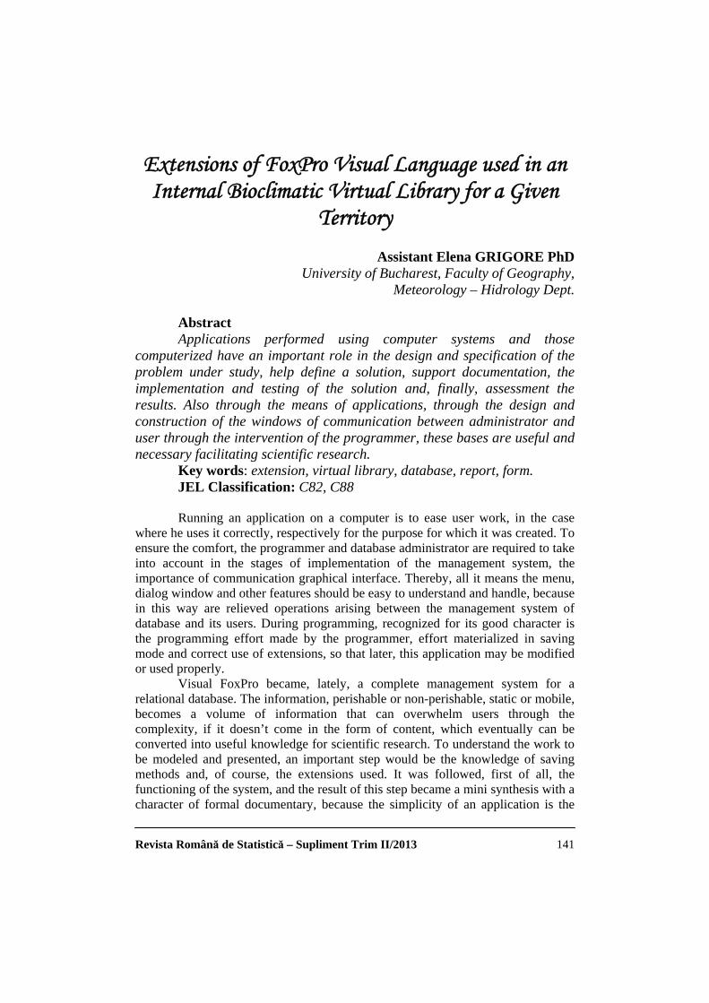
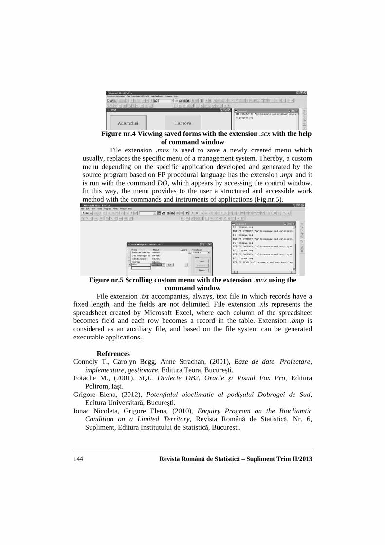
Extensions of FoxPro Visual Language used in an Internal Bioclimatic Virtual Library for a Given Territory .............................................................................. 141
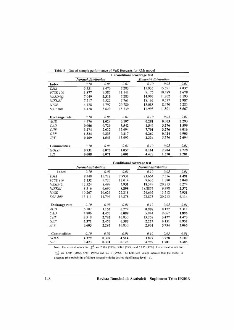
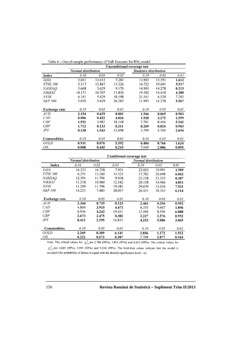
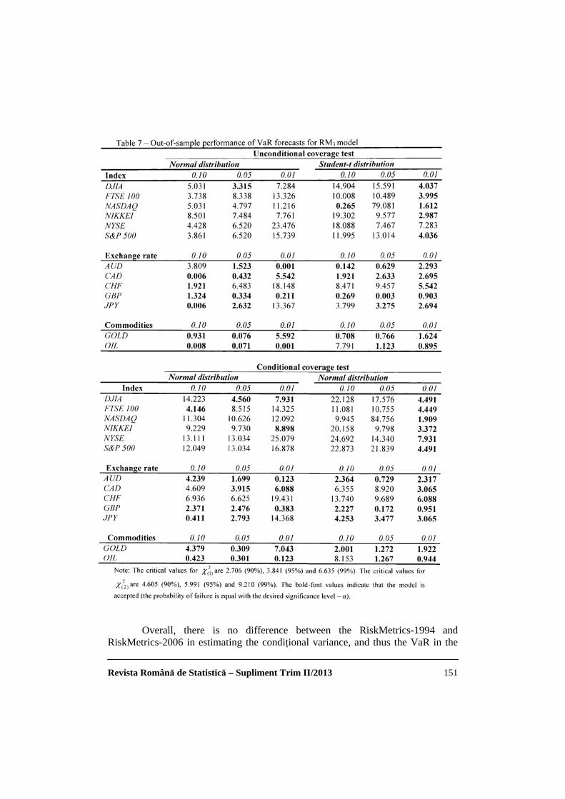
Assistant Elena GRIGORE PhD Analysis Based on the Risk Metrics Model........................................................................................................ 145
Lecturer Bogdan ZUGRAVU PhD Ec. Dumitru Cristian OANEA Prof. Victoria Gabriela ANGHELACHE PhD
Human Resources Management in Support of Improving the Adaptability of the Romanian Companies............................................ 155
Associate Professor Sorin Gabriel GRESOI PhD Associate Professor Aurelian DIACONU PhD Amelia DIACONU (EFTIMESCU) PhD Student
The Linear and Non-displaced Estimator in Multiple Regression ............................................................................ 161
Prof. Constantin ANGHELACHE PhD Prof. Vergil VOINEAGU PhD Assoc. prof. Alexandru MANOLE PhD Diana Valentina SOARE PhD Student Assistant teacher Ligia PRODAN PhD Student
Risk Management and Its Economic-Financial Importance............................................................................................... 167
Svetlana BRADUŢAN PhD Student
Revista Română de Statistică – Supliment Trim II/2013 10
General Aspects Regarding the Classical Hypotheses in Multiple Regression ............................................................................ 171
Prof. Constantin ANGHELACHE PhD Prof. Gabriela Victoria ANGHELACHE PhD Daniel DUMITRESCU PhD Student Ec. Cristi DUMITRESCU Adina Mihaela DINU PhD Student
International Production and Employment ......................................... 177 Assoc. prof. Anca-Mihaela TEAU PhD Lecturer Cristina Elena PROTOPOPESCU PhD
Securing European Integration ............................................................. 181 Prof. Constantin ANGHELACHE, PhD Valentin BICHIR, PhD Student Alex BODISLAV, PhD Student Andreea Gabriela BALTAC, PhD Student
The Price Policy of the Strategic Planning of the Enterprise.............. 185 Assoc. prof. Cristian - Marian BARBU PhD
Europe and the General Strategy .......................................................... 196 Prof. Constantin ANGHELACHE, PhD Valentin BICHIR, PhD Student Alex BODISLAV, PhD Student Ec. Bogdan DRAGOMIR Ec. Cristi DUMITRESCU
Brand Management in Business to Business Markets - Particularities of Business to Business Markets, Branding and Brand Equity - ................................................................ 200
Pareto’s Principle - Between Practical Validation and Scientific Deception - ............................................................................................... 205
Prof. Mircea UDRESCU PhD SME Branding......................................................................................... 219
Prof. Constantin CODERIE PhD Assoc. prof. Dan NASTASE PhD
Taxation – Important Role in Securing Budgetary Equilibrium........................................................................... 224
Prof. Radu Titus MARINESCU PhD
Revista Română de Statistică – Supliment Trim II/2013 11
Economic Growth: Concept, factors and Typology............................. 228 Prof. hon. Gheorghe MECU PhD
Judicial Capacity of the Commercial Entity - The Will of the Company ....................................................................... 233
Assoc. prof. Anca POPESCU-CRUCERU, PhD Student Assistant Eugenia-Gabriela LEUCIUC, PhD Student
Modeling Economic Growth .................................................................. 239 Lecturer Dragoş Gabriel MECU PhD
Analysis of State Budget Incomes During the Period 2010 – 2012 ............................................................................ 243
Assoc. prof. Raluca Andreea MIHALACHE PhD Foreign Direct Investments – a Solution a Sustainable Economic Development ............................................................................................ 248
State Intervention in Financial – Banking Environment in Order to Increase GDP........................................................................... 268
Daniel DUMITRESCU PhD Student Diana Valentina SOARE PhD Student
Public Property According to the New Civil Code .............................. 275 Lecturer Ioana Nely MILITARU PhD
Aspects Regarding Alternative Currencies .......................................... 283 Lecturer Andreia ROTARU PhD
Legal Proceedings and Modes that Must be Accessed by Enterprises Manufacturing Goods, Providing Works and Services in Time of Crisis ................................................... 292
Assoc. prof. Ilie GHEORGHE PhD Using Time Series in the Analysis of the Gross Domestic Product .................................................................................... 296
Contract Closing – Moment and Place of Closing Contracts by Electronic Means..................................................................................... 302
Lecturer Ioana Nely MILITARU PhD
Revista Română de Statistică – Supliment Trim II/2013 12
The Analysis of the Correlation Intensity Between Emerging Market During Economic Crisis.......................................... 307
Daniel ARMEANU Cristina Andreea DOIA Melania HANCILA Sorin CIOACA
Revista Română de Statistică – Supliment Trim II/2013 13
Democratic Participation in the Model for Emphasis and Protection of Cooperative Identity
and Social-Economic Activity of the Society
Ec. Sevastiţa GRIGORESCU
President of UCECOM Prof. Dan CRUCERU PhD
“Artifex” University of Bucharest
Abstract Cooperatives have always acted to allow people to gain access to
goods and services without being exploited. This involves doing business in compliance with a set of values based on what we call today sustainable development. By focusing on human needs, cooperatives respond to crises by contemporary sustainable development, delivering a distinct form of common values. Cooperatives seek to optimize the results for all intervenient, without pursuing the maximization of benefits for a single intervenient. To build an economic, social and ecological sustainable development is provisioned to be one the principal motivations and arguments of cooperative movement increase. This brings an answer to the question why cooperatives are necessary and beneficial in these historical circumstances. In simple terms, cooperatives are more effective than traditional business models.
Key words: model, value, intervenients, vision, crisis JEL Classification: P13, J54 Modelele economice tradiţionale suferă actualmente de o criză de
precaritate, în termeni economici, sociali şi ecologici. Criza financiară a fost un exemplu remarcabil de pericole privind favorizarea câştigului pe termen foarte scurt mai degrabă decât o viabilitate pe termen lung. Modelul capitalist dominant al ultimilor treizeci de ani a fost însoţit de o creştere a inegalităţilor, traducându-se printr-o diminuare a capitalului social şi a bunăstării. În acelaşi timp, căutarea valorii pentru acţionari a implicat foarte adesea sacrificarea protecţiei mediului, cum a fost cazul mareei negre din Golful Mexicului. Pentru mulţi, catastrofa aceasta a scos la iveală aceleaşi probleme „..o reglementare guvernamentală excesiv de tolerantă, beneficiile întreprinderii în ciuda riscurilor, o presă care s-a complăcut cu cei care au cauzat criza financiară. Marile bănci şi marile instituţii petroliere au în comun mai mult decât mărimea lor: Ce s-a întâmplat la Puţul Macondo.” (cf. New York Review of Books, 29 sept. 2011).
Revista Română de Statistică – Supliment Trim II/2013 14
Aceste crize sunt toate pornite dintr-un model de întreprindere care plasează randamentul financiar înaintea nevoilor umane, un model care caută să privatizeze câştigurile şi să repatrieze pierderile. Dar viitorul aparţine întreprinderilor care investesc în valori comune, care ţin cont de impactul lor asupra clienţilor, mediului, angajaţilor şi asupra viitorului.
Pe acest fond, Alianţa Cooperatistă Internaţională îşi propune să joace un rol preponderent în definirea unei viziuni a economiei cooperatiste, care să dea valoare rezultatelor pe termen lung şi repercusiunilor costuri/beneficii. În acelaşi timp, ea trebuie să se sprijine pe competenţele şi practicile cele mai bune la exteriorul mişcării cooperatiste, pentru a expune şi măsura diferitele forme de valoare pe care cooperativele le produc pentru societate şi pe care modelul capitalist dominant le produce într-o măsură dramatic insuficientă.
Ca obiectiv al asumării dezvoltării durabile, mişcarea cooperatistă îşi propune să demonstreze un angajament ferm către dezvoltarea durabilă, dar şi o contribuţie pozitivă la dezvoltarea durabilă pe trei direcţii, astfel:
a) În domeniul economic. Până acum întreprinderea deţinută de investitori s-a preocupat de interesul
acţionarilor, acţionând în interesul lor şi al unei mâini de intervenienţi. Dimpotrivă, cooperativele au numeroase mesaje pozitive de împărtăşit în legătură cu această problematică.
În primul rând, cooperativele financiare acţionează în interesul membrilor lor şi nu în cel al acţionarilor. Ele urmăresc o valoare pentru intervenienţi şi nu o valoare privilegiată pentru acţionari, ceea ce prin definiţie este mai puţin riscant. Aprecierile actuale sunt extrem de relevante: „Ne aflăm într-o situaţie în care proprietatea şi controlul băncilor sunt în general încredinţate unor agenţi reprezentând părţi infime din bilanţ, dar care funcţionează cu incitaţii la o asumare de risc ineficient din punct de vedere social. Perdanţii actualei crize financiare sunt evidenţi” (cf. Andy Haldane, Director General pentru Stabilitatea Financiară, Bank of England, http://www.Irb.co.uk/v34/n04/andrew-haldane/the-doom-loop), în timp ce „de-a lungul istoriei, cooperativele arată o tendinţă de rezistenţă la criză. Acelaşi lucru este valabil şi pentru criza actuală – băncile cooperatiste şi cooperativele de credit au avut rezultate mai bune în timpul crizei bancare actuale. De exemplu Rabobank a trecut la 42% din piaţa sa în 2008 şi instituţiile sale membre au beneficiat de o creştere de 20% a depozitelor. Nivelul de adeziune a cooperativelor de credit a crescut în cursul anilor 2008-09” (cf. J. Birchall & L. Ketilson, 2009, Rezilienţa modelului de afacere cooperatist în timp de criză. OIM.)
În al doilea rând, centrând activitatea întreprinderii pe serviciile şi nevoile umane, mai degrabă decât pe profit, cooperativele nu întâmpină aceeaşi problemă de viziune pe termen scurt care loveşte toate tipurile de societăţi financiare şi nefinanciare. În alţi termeni, ele nu suferă de problema financializării care a lovit capitalismul în cursul ultimilor douăzeci de ani, în care randamentul financiar este indicatorul principal al unei bune gestiuni. Ele ameliorează astfel diversitatea şi ecologia globală a formelor de întreprinderi, introducând o alegere veritabilă în
Revista Română de Statistică – Supliment Trim II/2013 15
maniera de a face afaceri. Cooperativele continuă să joace un rol important în viaţa economică a unor ţări. Spre exemplu, în „Canada: 1 canadian din 3 este membru al unui sistem de cooperative de credit” (cf. The Globe and Mail, 15/5/2012), sau „ Circa 250 milioane de agricultori în ţările dezvoltate fac parte dintr-o cooperativă (cf. Banca Mondială, Raport 2008 despre dezvoltarea mondială: Agricultura pentru dezvoltare), sau „În Kenya, cooperativele au angajate 300 000 persoane şi creează locuri de muncă indirecte pentru 2 milioane de persoane graţie capitalurilor şi oportunităţilor pe care le creează” (cf. OIM, 2012, Cum se reunesc femeile în cooperativele din Africa de Est).
b) În domeniul social. Printre efectele negative generate de capitalismul actual şi pe care statul
trebuie adesea să le rezolve se găsesc problemele sociale asociate individualismului şi inegalităţii. Unele dintre ele implică pur şi simplu suferinţe umane inutile. Altele generează costuri financiare pentru guverne , atunci când se manifestă sub forma unor probleme de sănătate şi criminalitate. Studii din domeniu sugerează că societăţile având un nivel ridicat de asociere a membrilor se situează mai bine din punct de vedere economic, asta în plus de faptul că profită de nivele de încredere şi participare democratică mai ridicată.
Cooperativele aduc o contribuţie foarte pozitivă în acest sens în două feluri:
Mai întâi, ele oferă servicii sociale acelora care sunt cei mai vulnerabili. Amploarea cooperativelor sociale variază de la o ţară la alta. Ele nu sunt numai simpli actori de piaţă, ci furnizează servicii care, în alte condiţii, ar trebui oferite de stat. În acest caz, statul are din punct de vedere fiscal tot interesul să le ajute, în special în cazul unei crize fiscale vizibile.
În al doilea rând, asocierea şi adeziunea sunt bunuri în sine, acţionând ca resurse importante cu ajutorul cărora societatea şi economia prosperă.
Cooperativele contribuie la rezerva de capital social al unei naţiuni, în proporţii pe care întreprinderile tradiţionale nu le egalează. Naţiunile Unite recunoaşte acest lucru, solicitând în acelaşi timp guvernelor să încurajeze şi să faciliteze crearea şi dezvoltarea cooperativelor, inclusiv prin luarea de măsuri care vizează acordarea posibilităţii, persoanelor care trăiesc în sărăcie sau care aparţin grupurilor vulnerabile să se angajeze, pe cale voluntară, în crearea şi dezvoltarea de cooperative.
c) În plan ecologic. Există un număr în continuă creştere de dovezi care demonstrează că
mediul cooperatist se caracterizează prin bilanţ ecologic excelent. Pentru aceasta există multe explicaţii. În primul rând, în calitate de organizaţii participative, preocupările privind rezultatele ecologice viitoare pot fi explicate simplu de către membri, fără a fi nevoie să fie calculate în termeni de retur pe investiţie. În al doilea rând, atunci când cooperativele sunt multipartite, capacitatea întreprinderilor de a produce efecte negative din punct de vedere ecologic este diminuată în raport cu a unui intervenient particular.
Revista Română de Statistică – Supliment Trim II/2013 16
Obiectivul general al dezvoltării durabile, cu cele trei braţe – economic, social şi ecologic – este posibil de atins, în măsura în care se desfăşoară acţiuni coordonate, de genul: • Inovaţii în materie de contabilitate: Există deja un număr mare de iniţiative
prin care organizaţii cooperatiste redau activitatea patrimonială prin forme antagoniste de evaluare. Multe din aceste forme de contabilitate sunt dezvoltate deja de cei care lucrează cu întreprinderi axate pe profit, pentru a le conduce la dezvoltarea metodelor lor de raportare dincolo de datele financiare. Dar cooperativele au mult de câştigat pentru că şi-au însuşit această metodologie de reflectare a activităţii, pe care-o utilizează ca mijloc de demonstrare a impactului lor pozitiv. La această formă de reflectare patrimonială, cooperativele sunt interesate şi de instrumente specifice în materie de contabilitate, ca: reflectarea în bilanţ triplu; abordarea tabloului de evaluare echilibrată, returul social de investiţie, raportul pe impactul social, măsurarea stării de bine etc.
• Adoptarea celor mai bune practici. Definirea şi difuzarea celor mai bune practici în materie de dezvoltare durabilă şi încurajarea adoptării acestora de către comunitatea cooperatistă.
• Studii de caz. Sunt foarte importante studiile de caz care se ocupă de impactul activităţii cooperatiste la educaţie, la comunităţi, la sănătate şi la alte domenii de interes public.
• Colectarea de dovezi. Pentru a demonstra decidenţilor publici contribuţia cooperativelor la dezvoltarea durabilă, analiza economică a efectelor pozitive a acţiunilor cooperatiste este preţioasă.
• Apărare în faţa publicului. Mesajul cooperativelor nu se mai poate limita la expresia controlului democratic al membrilor. El trebuie să includă acum o referinţă la dezvoltarea durabilă, în aşa fel încât să suscite interesul decidenţilor publici, al publicului larg şi, în mod deosebit, al tinerilor.
Dezvoltarea durabilă constituie o componentă a strategiei de transformare a mediului cooperatist ce catalizează raporturile dintre toate componentele Planului de Acţiune pentru un Deceniu Cooperatist.
Într-o lume care suferă de mari deficienţe în ceea ce priveşte reprezentarea democratică, cooperativele demonstrează cum se pot face afaceri nu numai într-un mod diferit, dar şi mai bine, nu numai în interes propriu, dar şi în interesul întregii societăţi. Cu toate acestea, pentru a difuza acest important mesaj, este necesar să se transmită diferenţa specifică. Acest lucru creează, pe lângă un puternic sentiment de identitate comună, şi un mesaj care poate fi identificat cu o marcă ce personalizează această formă de întreprindere în raport cu toate celelalte cu care coexistă.
Omenirea asistă la procese specifice prin care modelele de afaceri clasice sunt reimaginate sau redefinite, prin luarea în considerare şi a altor scopuri, decât cel de maximizare a profitului.
Revista Română de Statistică – Supliment Trim II/2013 17
În cadrul acestor procese, cooperativele dispun de un atu major, evidenţiat de principiile cooperatiste. Pe baza acestor principii, cooperativele nu par diferite graţie unei remodelări a imaginii lor, ci ele sunt creaţii fundamental diferite. Valorile lor de dezvoltare durabilă nu sunt pur şi simplu grefate pe un model de întreprindere clasică, ci structurează maniera în care sunt deţinute, gestionate, administrate şi evaluate. Astfel, cooperativele au o autenticitate pe care nici-un alt model etic nu-l poate egala.
Măsura în care principiile cooperatiste, clar exprimate în Declaraţia Alianţei Cooperatiste Internaţionale, sunt aplicate sau nu, variază considerabil de la un sistem juridic la altul. De aceea, Provocarea 2020 consideră că este nevoie de un mesaj clar şi lipsit de orice confuzie. Într-o manieră generală, identitatea desemnează ceea ce reprezintă cooperativele pentru mişcarea cooperatistă şi pentru membrii săi, iar mesajul reprezintă desemnează maniera în care identitatea cooperatistă este prezentată şi difuzată mediului social şi economic, prin marketing specific, relaţii publice, logouri şi toate celelalte forme de comunicare cu persoanele din exteriorul mişcării cooperatiste.
Există suficiente puncte de vedere care sprijină adoptarea politicilor de marcă, în sensul construirii unor mărci cooperatiste. Dar există şi opinii care consideră marca ca o asociere cu drepturile de proprietate intelectuală, desemnând imagini atrăgătoare pentru consumatori. Deoarece niciuna din aceste semnificaţii nu este coerentă cu o mişcare care crede cu fermitate în valori ce se înscriu în durată şi care doreşte să încurajeze o generalizare a utilizării noţiunii de cooperativă ce se vrea disponibilă în mod gratuit pentru toţi cei care doresc să-i urmeze principiile, ideea centrării pe marcă se pare că nu are prea mulţi susţinători.
Ca atare, mişcarea are un interes legitim să protejeze integritatea cuvântului cooperativă pentru ca acesta să nu fie utilizat în sens peiorativ. De aceea, Planul de Acţiune pentru un Deceniu Cooperatist caută să proiecteze în aceeaşi măsură participare şi dezvoltarea durabilă prin mesajul cooperatist. Anul Internaţional al Cooperativelor al ONU şi logo-ul care l-a însoţit au demonstrat aspectele pozitive ale difuzării unui mesaj distinctiv unic pentru mişcare, care să fie difuzat în sfere multiple. Numele de domeniu.coop. furnizează, de asemenea, oportunitatea unei distincţii clare.
Atingerea obiectivului de consolidare a identităţii cooperatiste presupune acţiuni concertate, de genul: • Diseminarea, prin toate mijloacele, a Declaraţiei privind Identitatea
Cooperatistă şi îmbogăţirea conţinutului acesteia prin Directive regionale, care să conţină neapărat nucleul dur al principiilor ce dau consistenţă mişcării cooperatiste la nivel mondial..
• Constituirea unui cadru de reglementări care să facă posibilă utilizarea numelui de domeniu.coop numai de cei care satisfac cerinţele cadru cuprinse în Declaraţia privind Identitatea Cooperatistă. Pentru acest deziderat, Alianţa Cooperatistă Internaţională trebuie să lucreze cu organismele naţionale şi cu guvernele naţionale atunci când se constată dificultăţi în prevalarea principiilor generale cooperatiste.
Revista Română de Statistică – Supliment Trim II/2013 18
• Asigurarea unei unităţi de reprezentare a vocii cooperatiste în dezbaterea politică mondială, nu numai pe baza principiilor comune de funcţionare, ci şi printr-un semn comun al adeziunii lor. Amploarea cu care logo-ul AIC 2012 a fost adoptat de către societăţi a demonstrat forţa identificării cu valori comune dincolo de frontierele naţionale.
• Conceperea de mesaje care să funcţioneze în interesul cooperativelor pe termen lung. După dezvoltarea de Directive trebuie pusă la punct o frazeologie corespunzătoare, inteligibilă din punctul de vedere al difuzării mesajului.
• Promovarea mai largă a identităţii cooperatiste în şcoli de comerţ şi în organizaţii profesionale de resort.
Pe linia identităţii, Planul de Acţiune pentru un Deceniu Cooperatist propune ca, în anii următori, mişcarea să facă în aşa fel încât cooperativele să fie asimilate atât participării cât şi dezvoltării durabile, proces care include recunoaşterea securităţii financiare a instituţiilor financiare cooperatiste, dar şi contribuţia lor la securitatea socială locală şi mondială.
Acest capitol structural este legat de celelalte teme după cum urmează: identitatea trebuie să fie alimentată cu temele participare şi dezvoltare durabilă, dar identitatea trebuie să le considere drept caracteristici distincte; identitatea trebuie să precizeze tipul de capital utilizat pentru finanţarea cooperativelor, iar caracterul distinctiv al capitalului cooperatist în raport cu capitalul tradiţional trebuie să joace un rol important în difuzarea identităţii cooperatiste; identitatea cooperatistă trebuie să fie recunoscută într-un cadru legal.
Este evident că procesul de formare de noi cooperative ţine contextul legislativ existent în fiecare ţară, iar viziunea că, asociaţiile cooperatiste sunt o formă de întreprindere marginală este încă des întâlnită. De asemenea, există o incapacitate în a înţelege cum funcţionează cooperativele şi care sunt avantajele de care acestea dispun. La aceşti factori contribuie la faptul că structurile financiare, juridice şi administrative sunt concepute de cea mai mare majoritate a întreprinderilor care sunt axate pe profit şi sunt deţinute de acţionari.
În această direcţie, rezoluţii ale ONU, Declaraţia Finală a Conferinţei de la Veneţia din 2012, recomandări ale OIM solicită guvernelor încurajarea şi facilitarea creării de cooperative. Spre exemplu, din unele recomandări ale OIM rezultă cerinţe, de genul: guvernele să furnizeze o politică şi un cadru legal coerent cu natura şi funcţia cooperativelor şi fondat pe valorile şi principiile cooperatiste; adoptarea de măsuri vizând promovarea potenţialului cooperativelor în toate ţările, oricare ar fi nivelul lor de dezvoltare pentru o serie de obiective dintre care crearea de activităţi generatoare de venituri şi locuri de muncă, dezvoltarea capacităţilor resurselor umane şi cunoaşterea cooperaţiei, dezvoltarea potenţialului întreprinderilor, creşterea economiei şi investiţiei şi ameliorarea bunăstării sociale şi economice; promovarea de cooperative ca unul dintre pilonii dezvoltării economice şi sociale naţionale şi internaţionale; guvernele să faciliteze accesul cooperativelor la servicii de ajutorare, la intervenţii financiare şi de credit etc.
Revista Română de Statistică – Supliment Trim II/2013 19
Mişcarea cooperatistă nu îşi propune o campanie legislativă care să încline balanţa respectivă în favoarea sa, dar caută ca guvernele şi instituţiile legislative să înţeleagă bine avantajele economice şi sociale ale cooperaţiei şi să sprijine tendinţele de formare şi funcţionare de noi cooperative printr-un cadru legislativ adecvat.
Demersurile Alianţei Cooperatiste Internaţionale trebuie să fie acelea de a produce dovezi ale valorii publice şi ale perenităţii cooperativelor, care întăresc argumentul de reformă guvernamentală în favoarea cooperativelor, în special într-o perioadă de criză financiară în care multe state caută forme noi de securitate socială.
Un asemenea obiectiv poate fi atins prin acţiuni de genul: crearea unei reţele internaţionale pentru birourile de înregistrare şi organismele de reglementare; dezvoltarea directivelor privind maniera de aplicare a Principiilor cooperaţiei; integrarea programului cooperatist în instituţiile mondiale de dezvoltare; dezvoltarea capacităţii de a răspunde la oportunităţile create pentru cooperative prin evenimente şi schimbări politice mondiale şi regionale; publicarea de dovezi despre avantajele sociale şi publice ale cooperativelor; crearea unui mijloc de acţiune pentru a evalua cadrele legale naţionale ce vizează activitatea cooperatistă etc.
Un cadru legal favorabil este necesar pentru: a integra, permite şi favoriza sistemele de participare, a sigura stabilitatea juridică a cooperativelor pentru întărirea perenităţii lor, a proteja şi susţine identitatea cooperatistă, a permite introducerea de forme corespunzătoare de capital. Toate aceste cerinţe ilustrează şi legăturile cadrului legal cu celelalte componente ale strategiei de acţiune.
Întreprinderile nu pot funcţiona fără capital şi cooperativele nu pot face abstracţie de la această cerinţă. Chiar dacă au capacitatea de a împrumuta, ele au nevoie să-şi finanţeze activităţile pe termen lung, pentru care ele au, în general, de o anumită formă de capital cu un risc pe termen lung. Capitalul cooperativelor provine în general de la membri prin intermediul capitalului social sau al beneficiilor nerepartizate. Prin definiţie, beneficiile nerepartizate cer timp pentru a fi acumulate şi , evident, nu pot fi disponibile la demararea activităţii. Cu mulţi ani în urmă, la începuturile activităţii cooperatiste, acestea erau finanţate prin depozite în bani gheaţă ale membrilor, în perioada în care nu existau bănci, iar cetăţenii îşi păstrau economiile la cooperative, putând fi retrase la nevoie.
Capitalul social disponibil (care poate fi retras) nu a mai fost în măsură să acopere capitalul necesar, pe măsură ce oamenii au apelat tot mai mult la alte forme de servicii financiare, nemaiavând nevoie de cooperative ca forme de refugiu pentru banii disponibili.
Întreprinderile deţinute de investitori dezvoltă capitaluri atrăgând pe cei care sunt interesaţi de un anumit retur financiar în termeni de dividende, de creştere a valorii capitalului împrumutat pe o perioadă de timp, sau o combinaţie a celor două. Fondurile proprii tradiţionale oferă aceste avantaje, ele fiind bazate pe principiul că deţinerea unei acţiuni conferă investitorului o parte proporţională a
Revista Română de Statistică – Supliment Trim II/2013 20
valorii potenţiale a capitalului societăţii şi o cotă-parte a beneficiilor distribuite sub formă de dividende.
Capitalul cooperatist este diferit. Mai întâi, un membru nu poate retrage, în general, din societate decât valoarea sumelor depuse sau subscrise prin părţi. Nu există deci nici un drept asupra unei părţi din valoarea potenţială. În al doilea rând, chiar dacă cooperativele pot plăti dobânzi pe capital, conform celui de-al treilea principiu cooperatist membrii primesc o remuneraţie limitată, dacă este cazul, din capitalul subscris, ca o condiţie a adeziunii lor. În măsura în care profiturile sau excedentele sunt distribuite membrilor, repartizarea este proporţională cu schimburile membrilor cu societatea. În comparaţie cu fondurile proprii ale unei întreprinderi tradiţionale, capitalul cooperatist nu oferă investitorilor avantaje economice comparabile. În consecinţă, nu este la fel de interesant din punct de vedere financiar şi prezintă un interes mic din partea investitorilor.
Planul de Acţiune pentru un Deceniu al Cooperativelor şi Provocarea 2020 încearcă să facă mediul cooperatist atractiv, prin a face să corespundă nevoia cetăţenilor de a avea un loc sigur de a păstra banii disponibili pe moment, dar necesari mai târziu, cu nevoile întreprinderilor de a crea bunuri necesare tot cetăţenilor.
Istoria ultimilor 150 de ani a constat în a transforma oamenii în investitori, prin a plasa banii în locuri care să le aducă cele mai bune profituri. A maximiza randamentul economiilor proprii este acum normă generală. Dar acesta este modelul care a devenit falimentar şi căruia economia cooperatistă îi oferă o alternativă. În acest proces, nu numai întreprinderea trebuie să se schimbe, ci şi oamenii. Ei trebuie să înceteze în a se comporta ca investitori care caută să maximizeze câştigurile, ci ca oameni responsabili în a construi o lume durabilă, funcţională. Omenirea trăieşte o epocă de mari schimbări, în care comportamentele populare şi motivaţiile se schimbă.
Ca atare, instrumentele financiare trebuie să fie în armonie cu comportamentele şi motivaţiile actuale. Sistemul cooperatist reprezintă o propunere financiară care prevede un retur de investiţii, fără a distruge identitatea cooperatistă şi care permite oamenilor să acceadă la fondurile lor atunci când au nevoie.
În acest context, instrumentele financiare corespunzătoare, prin care oamenii pot finanţa cooperativele, sunt esenţiale. Este nevoie de instrumente care să permită plasarea şi retragerea uşoară a banilor din cooperative, şi care: să ofere o bază stabilă pentru activităţile cooperativei, să ofere o ieşire adaptată persoanelor care oferă bani (comanditarilor) şi să nu compromită natura cooperativei, controlul exercitat de membrii cooperatori şi angajamentul lor către natura cooperatistă.
Pentru atingerea obiectivului sunt necesare acţiuni diverse, între care se regăsesc: promovarea şi încurajarea de manieră generală a finanţării cooperativelor de către membrii actuali, formularea de propuneri clare către potenţialii comanditari, dezvoltarea unui instrument financiar generic modern care să fie catalogat drept capital-risc, dezvoltarea unei serii de variante pentru acest model generic pentru a conveni asupra diferitelor categorii de cooperative, identificarea
Revista Română de Statistică – Supliment Trim II/2013 21
de instituţii care pot acţiona ca strângători sau intermediari pentru organizaţiile cooperatiste, utilizarea Fondului Mondial de Dezvoltare de Cooperative pentru a încuraja crearea de noi instrumente financiare, examinarea riscurilor şi oportunităţilor create de utilizarea de filiale şi alte dispozitive de structură de grup, crearea unui indice cooperatist specific pentru a măsura creşterea şi performanţă, crearea de norme contabile care ţin cont de caracteristicile unice ale modelului cooperatist, accelerarea comerţului mondial între cooperative graţie dispozitivelor de curtaj şi a structurilor de servicii partajate etc.
Capitalul este legat cu celelalte teme după cum urmează: capitalul este fundamental legat de identitate – el informează despre însăşi natura identităţii cooperatiste şi trebuie să fie o caracteristică distinctivă ilustrând modul cum sunt diferite cooperativele de entităţi care maximizează profitul; această identitate este ea însăşi fondată pe caracteristicile de bază ale participării şi dezvoltării durabile, care trebuie să treacă prin identitate pentru a atrage capitaluri; dar forma de capital trebuie repusă în cadru legal.
Concluzii Planul de Acţiune pentru un Deceniu al Cooperativelor şi Provocarea 2020
sunt cu adevărat ambiţioase. Ideile noii mişcări cooperatiste oferă o alternativă oamenilor, răspunzând nevoilor acestora tocmai când se simt abandonaţi de întreprinderea tradiţionalistă.
Astăzi toată lumea are nevoie de aceste idei. Comunitatea mondială este cea care a fost abandonată prin maniera tradiţională de a face afaceri, în care profiturile şi creşterea sunt mai importante decât dezvoltarea durabilă şi interesul unor persoane este mai important decât interesul tuturor. De aceea, acest Plan de Acţiune este unul ambiţios pentru a clarifica mesajul cooperatist şi a-l difuza unei comunităţi mondiale care, actualmente, nu-şi mai imaginează sigur viitorul.
Dar pentru ca acest Plan de Acţiune să fie credibil şi eficient, el trebuie adoptat de către instanţele naţionale, societăţile individuale, de toate persoanele care cred în maniera cooperatistă de a face afaceri. Prin acţiunea colectivă se edifică Provocarea 2020.
Bibliografie selectivă
Cruceru, D. (2012) – „Cooperaţia în România. Istorie şi actualitate”, Editura Artifex, Bucureşti
www.ica.coop
Revista Română de Statistică – Supliment Trim II/2013 22
Inflation and Unemployment – a Correlative Analysis
Prof. Constantin ANGHELACHE PhD
„Artifex” University of Bucharest/ Academy of Economic Studies of Bucharest
Prof. Vergil VOINEAGU PhD Academy of Economic Studies of Bucharest
Mihai GHEORGHE PhD Ec. Cristina SACALĂ
National Institute of Statistics Ec. Ionuţ NEGOIŢĂ
Manager Ec. Alexandru URSACHE
Abstract The economic and financial crisis considered within the national
behavior, within the behavior implied by the one involved by the overlapped context, within the mixed and overlapped behavior, both national and international (and vice-versa), proved that each country and the European Union as well are facing a series of structural issues such as: the domestic economic growth, the lack of productivity, the high rate of the unemployment, the volatility of the inflation and its impact, the high levels of the debt and deficit etc. To all these sectorial issues, one has to add the interdependence/static and dynamic correlation between the national macroeconomic unbalances and, mainly, its impact. This is the context in which the interdependence/statistical correlation between inflation and unemployment should be considered. Key words: inflation, estimator, unemployment, interdependence, monetary
JEL Classification: E24, E31 In the frame of the modern sectorial and macroeconomic statistics, the undertaken approach has the role of establishing behaviors over ex-post periods, to validate or invalidate the various hypotheses ex-ante set up and, consequently, to substantiate decisions and even policies. In this whole approach, the statistics resort to measurable notions, such as tendencies, estimators, estimates etc. Objectively
Revista Română de Statistică – Supliment Trim II/2013 23
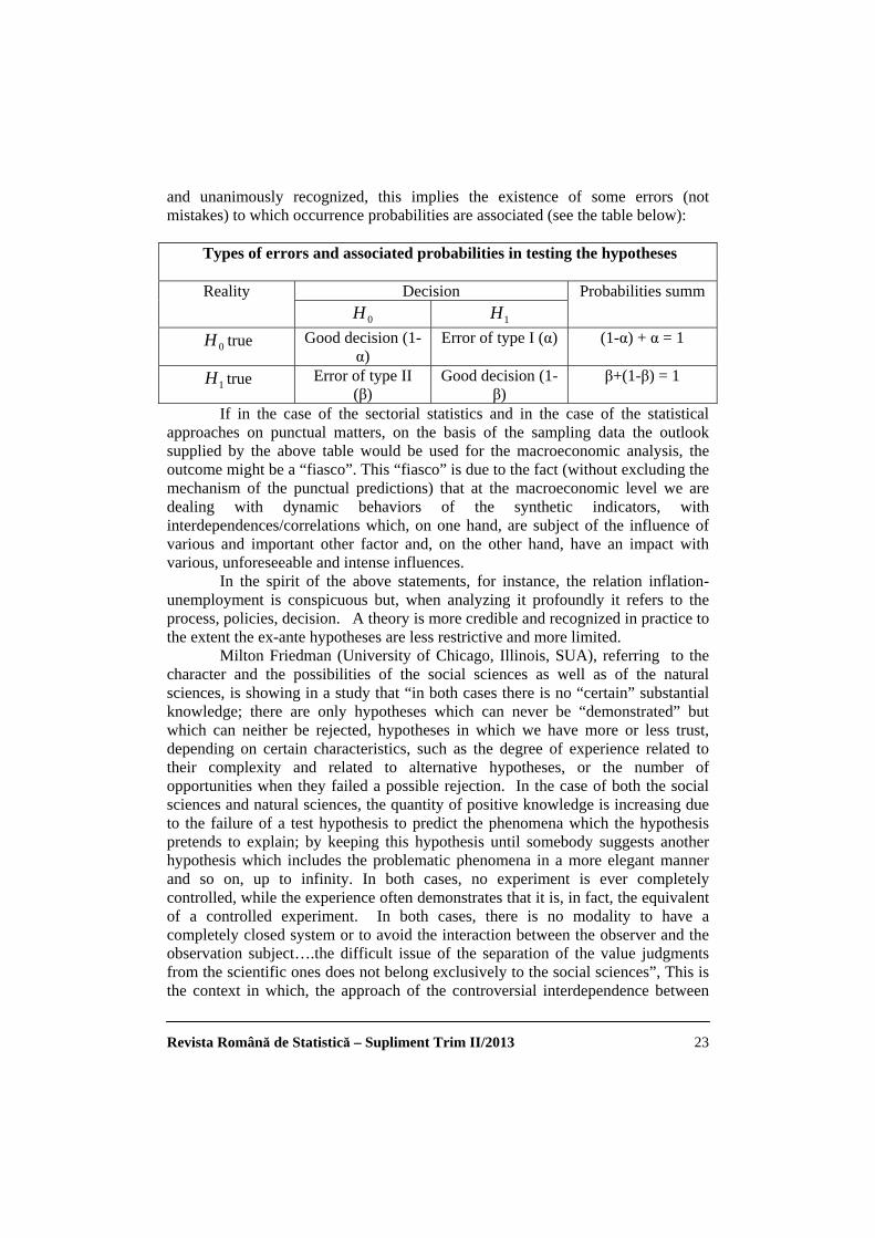
and unanimously recognized, this implies the existence of some errors (not mistakes) to which occurrence probabilities are associated (see the table below):
Types of errors and associated probabilities in testing the hypotheses
Decision Reality 0H 1H
Probabilities summ
0H true Good decision (1-α)
Error of type I (α) (1-α) + α = 1
1H true Error of type II (β)
Good decision (1-β)
β+(1-β) = 1
If in the case of the sectorial statistics and in the case of the statistical approaches on punctual matters, on the basis of the sampling data the outlook supplied by the above table would be used for the macroeconomic analysis, the outcome might be a “fiasco”. This “fiasco” is due to the fact (without excluding the mechanism of the punctual predictions) that at the macroeconomic level we are dealing with dynamic behaviors of the synthetic indicators, with interdependences/correlations which, on one hand, are subject of the influence of various and important other factor and, on the other hand, have an impact with various, unforeseeable and intense influences. In the spirit of the above statements, for instance, the relation inflation-unemployment is conspicuous but, when analyzing it profoundly it refers to the process, policies, decision. A theory is more credible and recognized in practice to the extent the ex-ante hypotheses are less restrictive and more limited. Milton Friedman (University of Chicago, Illinois, SUA), referring to the character and the possibilities of the social sciences as well as of the natural sciences, is showing in a study that “in both cases there is no “certain” substantial knowledge; there are only hypotheses which can never be “demonstrated” but which can neither be rejected, hypotheses in which we have more or less trust, depending on certain characteristics, such as the degree of experience related to their complexity and related to alternative hypotheses, or the number of opportunities when they failed a possible rejection. In the case of both the social sciences and natural sciences, the quantity of positive knowledge is increasing due to the failure of a test hypothesis to predict the phenomena which the hypothesis pretends to explain; by keeping this hypothesis until somebody suggests another hypothesis which includes the problematic phenomena in a more elegant manner and so on, up to infinity. In both cases, no experiment is ever completely controlled, while the experience often demonstrates that it is, in fact, the equivalent of a controlled experiment. In both cases, there is no modality to have a completely closed system or to avoid the interaction between the observer and the observation subject….the difficult issue of the separation of the value judgments from the scientific ones does not belong exclusively to the social sciences”, This is the context in which, the approach of the controversial interdependence between
Revista Română de Statistică – Supliment Trim II/2013 24
the two major macroeconomic unbalances, with a particular impact, such as inflation and unemployment, must be integrated.
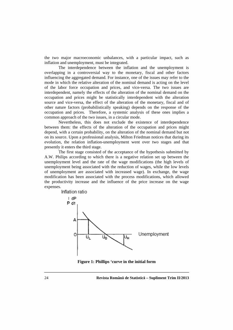
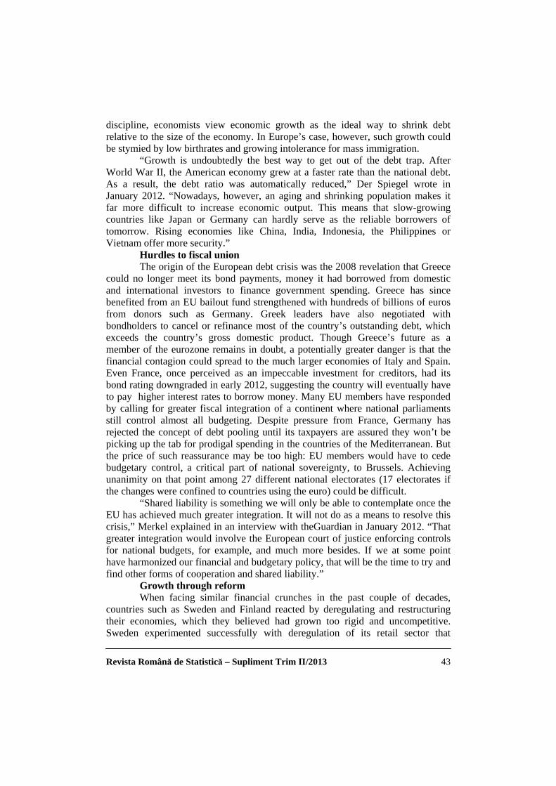
The interdependence between the inflation and the unemployment is overlapping in a controversial way to the monetary, fiscal and other factors influencing the aggregated demand. For instance, one of the issues may refer to the mode in which the relative alteration of the nominal demand is acting on the level of the labor force occupation and prices, and vice-versa. The two issues are interdependent, namely the effects of the alteration of the nominal demand on the occupation and prices might be statistically interdependent with the alteration source and vice-versa, the effect of the alteration of the monetary, fiscal and of other nature factors (probabilistically speaking) depends on the response of the occupation and prices. Therefore, a systemic analysis of these ones implies a common approach of the two issues, in a circular mode. Nevertheless, this does not exclude the existence of interdependence between them: the effects of the alteration of the occupation and prices might depend, with a certain probability, on the alteration of the nominal demand but not on its source. Upon a professional analysis, Milton Friedman notices that during its evolution, the relation inflation-unemployment went over two stages and that presently it enters the third stage. The first stage consisted of the acceptance of the hypothesis submitted by A.W. Philips according to which there is a negative relation set up between the unemployment level and the rate of the wage modifications (the high levels of unemployment being associated with the reduction of wages, while the low levels of unemployment are associated with increased wage). In exchange, the wage modification has been associated with the process modifications, which allowed the productivity increase and the influence of the price increase on the wage expenses.
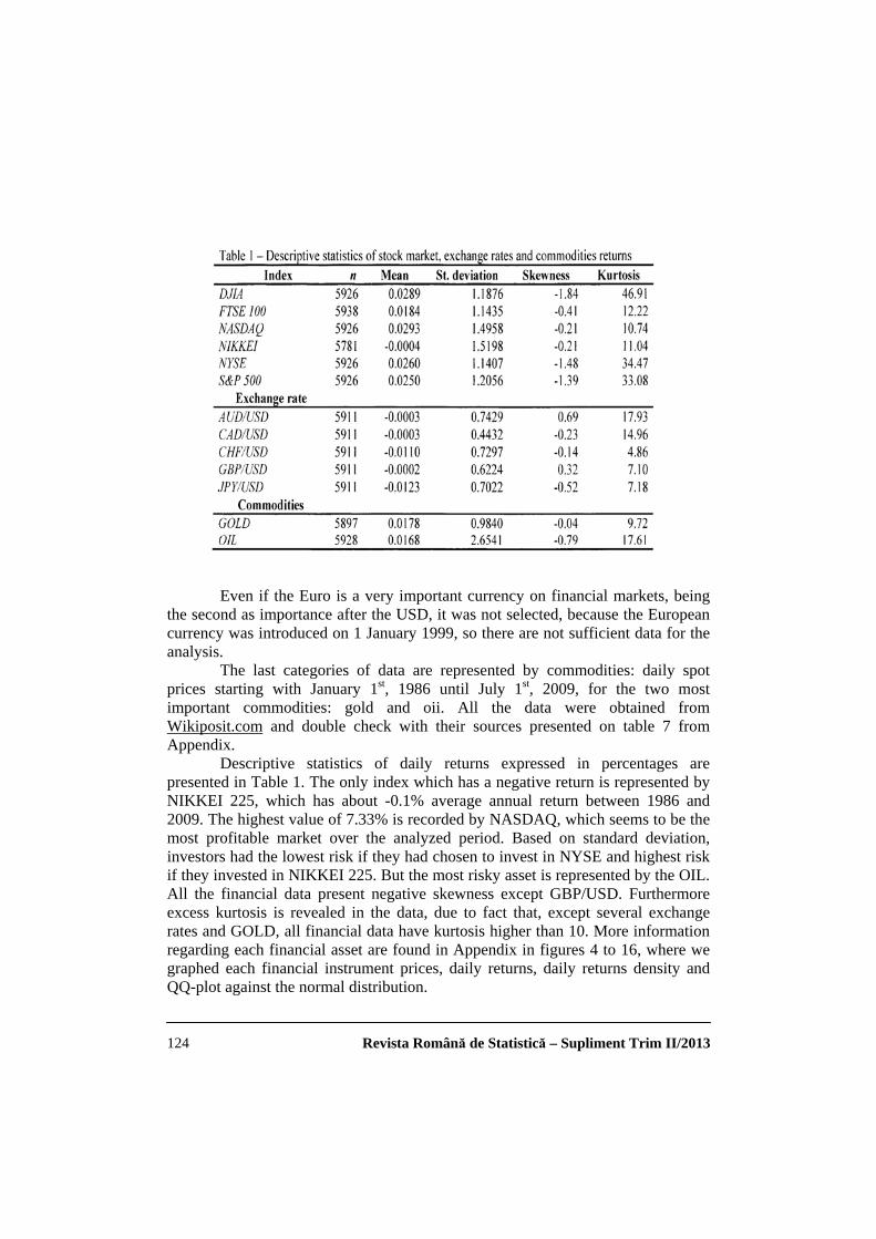
Figure 1: Phillips ‘curve in the initial form
Revista Română de Statistică – Supliment Trim II/2013 25
The economists have analyzed the Phillips’ curve on statistical data from different countries and periods of time and came to the conclusion that Phillips’ hypothesis/curve is not constantly stable: the inflation rate corresponding to a certain rate of the unemployment did not hold fix; the inflation rates which, at the beginning, corresponded to the low levels of the unemployment occurred in fact in the conditions of high levels of unemployment etc. The instability of the Phillips’ curve can be explained by the impact of the non-anticipated alterations of the nominal demand on the markets, characterized (directly or indirectly) by long-term committments as far as both the capital and the labor force are concerned (alternative opportunities for the labor force occupation, the cost for an employee may increase for the alternative employers etc.)
In other terms, “The long-term commitments in the sphere of the labor force can be explained by the cost of getting information concerning the employees for the employers and, for the employees, the cost of getting information concerning the alternative opportunities of occupation, plus the specific human capital which makes that, for an employer, the value of an employee increases in time exceeding thus the value for other potential employers.
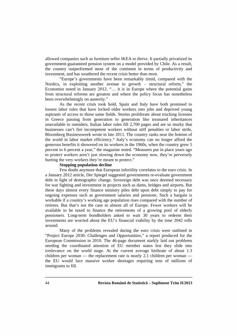
This might be interpreted as follows: there is not an automatic compensation of the market but only a delayed adjustment of the prices and quantities as response to the demand or offer alteration (for instance, in the case of the real estate renting market). Meantime, the commitments (targets) set up depend not only on the prices currently observed but also on the forecasted prices over the entire period of the commitments volatility. Consequently, it is compulsory (M. Friedman,...), that in the analysis of the relation between the inflation and the unemployment, the distinction between the effects on short term and those on long term of the non-anticipated modifications of the nominal demand is made. An increase of the nominal wages may be perceived by the employees as a real salaries increase and, as a consequence, an increase of the offer is induced, while the employers perceive a reduction of the real wages which induces an increase of the offer of jobs.
Figure 2: Adjusted Phillips’ curve
Revista Română de Statistică – Supliment Trim II/2013 26
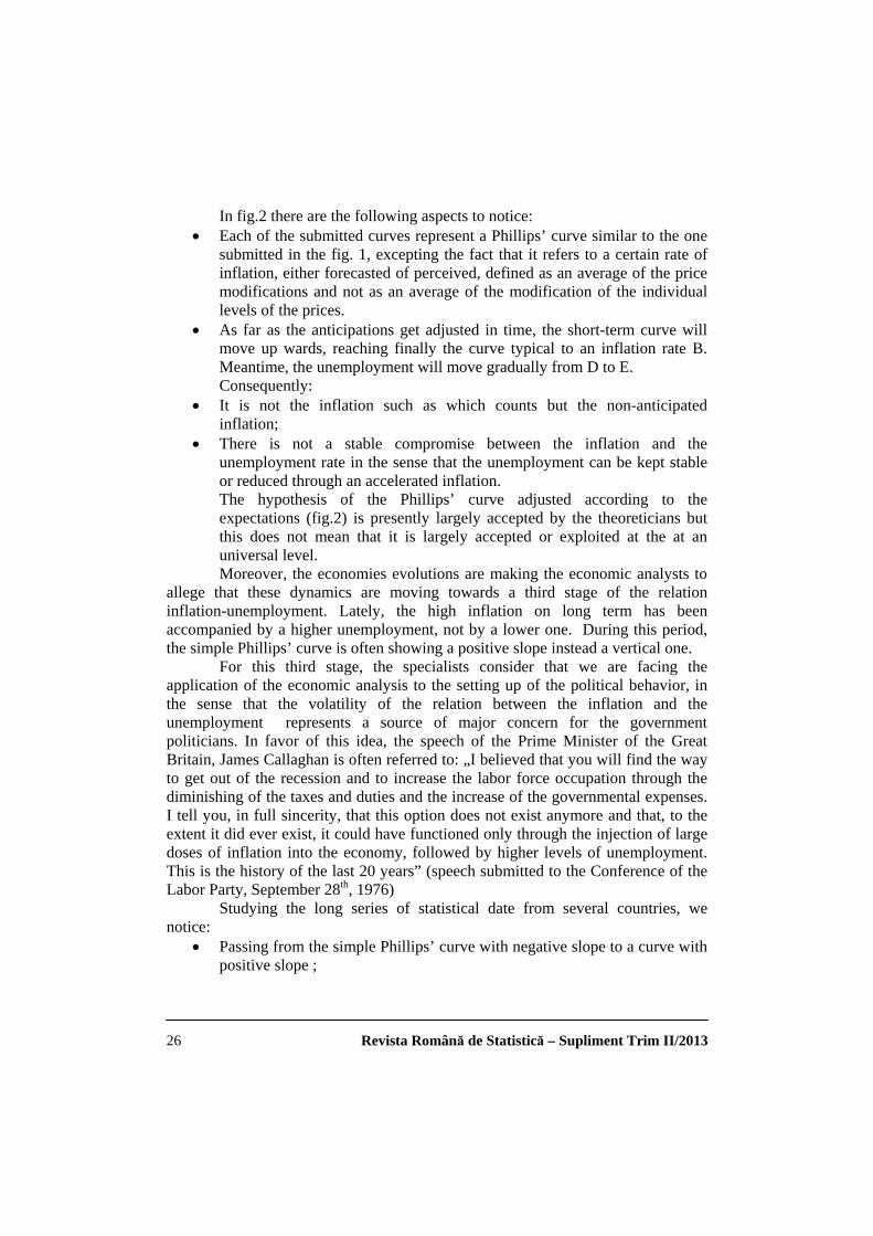
In fig.2 there are the following aspects to notice: • Each of the submitted curves represent a Phillips’ curve similar to the one
submitted in the fig. 1, excepting the fact that it refers to a certain rate of inflation, either forecasted of perceived, defined as an average of the price modifications and not as an average of the modification of the individual levels of the prices.
• As far as the anticipations get adjusted in time, the short-term curve will move up wards, reaching finally the curve typical to an inflation rate B. Meantime, the unemployment will move gradually from D to E. Consequently:
• It is not the inflation such as which counts but the non-anticipated inflation;
• There is not a stable compromise between the inflation and the unemployment rate in the sense that the unemployment can be kept stable or reduced through an accelerated inflation. The hypothesis of the Phillips’ curve adjusted according to the expectations (fig.2) is presently largely accepted by the theoreticians but this does not mean that it is largely accepted or exploited at the at an universal level.
Moreover, the economies evolutions are making the economic analysts to allege that these dynamics are moving towards a third stage of the relation inflation-unemployment. Lately, the high inflation on long term has been accompanied by a higher unemployment, not by a lower one. During this period, the simple Phillips’ curve is often showing a positive slope instead a vertical one. For this third stage, the specialists consider that we are facing the application of the economic analysis to the setting up of the political behavior, in the sense that the volatility of the relation between the inflation and the unemployment represents a source of major concern for the government politicians. In favor of this idea, the speech of the Prime Minister of the Great Britain, James Callaghan is often referred to: „I believed that you will find the way to get out of the recession and to increase the labor force occupation through the diminishing of the taxes and duties and the increase of the governmental expenses. I tell you, in full sincerity, that this option does not exist anymore and that, to the extent it did ever exist, it could have functioned only through the injection of large doses of inflation into the economy, followed by higher levels of unemployment. This is the history of the last 20 years” (speech submitted to the Conference of the Labor Party, September 28th, 1976) Studying the long series of statistical date from several countries, we notice:
• Passing from the simple Phillips’ curve with negative slope to a curve with positive slope ;
Revista Română de Statistică – Supliment Trim II/2013 27
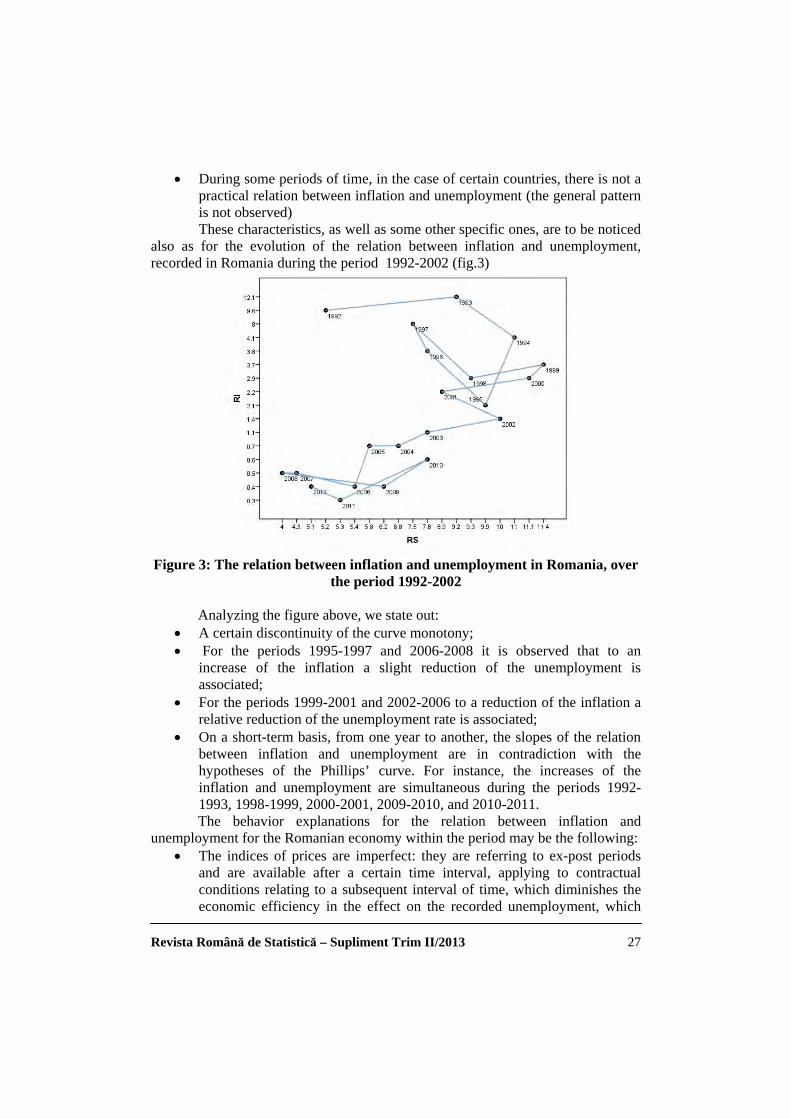
• During some periods of time, in the case of certain countries, there is not a practical relation between inflation and unemployment (the general pattern is not observed) These characteristics, as well as some other specific ones, are to be noticed
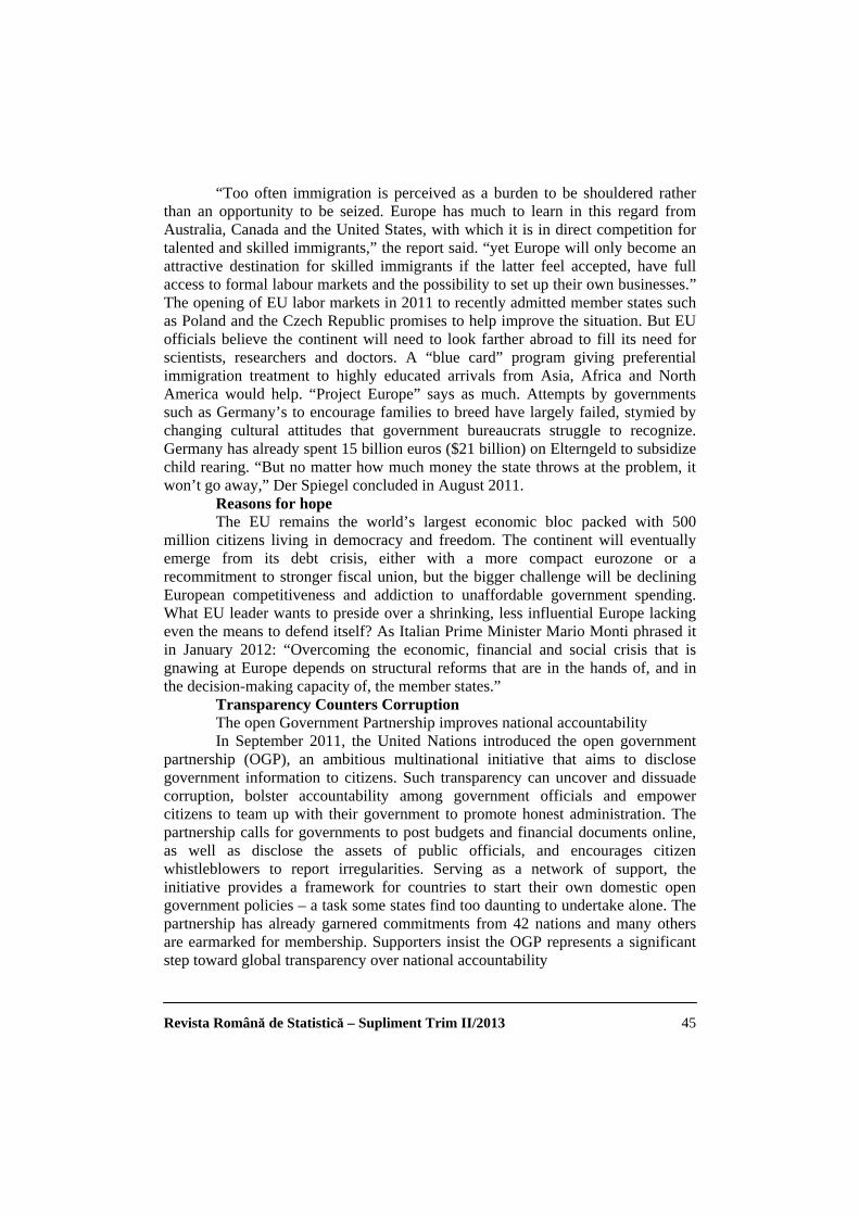
also as for the evolution of the relation between inflation and unemployment, recorded in Romania during the period 1992-2002 (fig.3)
Figure 3: The relation between inflation and unemployment in Romania, over
the period 1992-2002
Analyzing the figure above, we state out: • A certain discontinuity of the curve monotony; • For the periods 1995-1997 and 2006-2008 it is observed that to an
increase of the inflation a slight reduction of the unemployment is associated;
• For the periods 1999-2001 and 2002-2006 to a reduction of the inflation a relative reduction of the unemployment rate is associated;
• On a short-term basis, from one year to another, the slopes of the relation between inflation and unemployment are in contradiction with the hypotheses of the Phillips’ curve. For instance, the increases of the inflation and unemployment are simultaneous during the periods 1992-1993, 1998-1999, 2000-2001, 2009-2010, and 2010-2011. The behavior explanations for the relation between inflation and
unemployment for the Romanian economy within the period may be the following: • The indices of prices are imperfect: they are referring to ex-post periods
and are available after a certain time interval, applying to contractual conditions relating to a subsequent interval of time, which diminishes the economic efficiency in the effect on the recorded unemployment, which
Revista Română de Statistică – Supliment Trim II/2013 28
may be a masked one. The commitments on short-term might lead to a more rapid adjustment of the labor force occupied under to modified conditions and hence a lower unemployment, while a delay in adjusting the duration of the commitments might lead to a high unemployment. In other words, a slow adjustment of the commitments and the imperfections of the indexation may contribute to the recording of an increase of the unemployment.
• Another explanation is connected with the impact of the inflation volatility on the information required by the economic agents in order to decide what and how to produce or how to utilize the resources. The relevant information refers to the relative prices of a product as against another one, of the services of a certain production factor as against a different one, of the products relating to the factors services, of the today prices as against the prices of the forthcoming periods. More volatile the general inflation rate is, more difficult is to extract the signal referring to the relative prices, due to the increase of the “noise” of the market signals, at least during the periods when the institutional commitments are not accommodated to the new situations. These effects of the increased volatility of the inflation can occur even in the conditions of an existing legal frame for price adjustment. In the case of the modern society, the government itself is a producer of services sold on the market: from the postal services to a large scale of other services. This means that a weight relatively large comparatively with the European level, of the prices/tariffs is regulated by government decisions: from the transport tariffs up to the tariffs applied to the electricity and natural gas. On the other side, the inflation volatility makes the social and political forces as well as the trade unions to ask the governments to take adequate steps in order to control the inflation. Of course, the details differ from one country to another, from one period to another but there is a certain aspect to consider, namely the fact that the distortions within the relative prices evolution are largely due to the market frictions and the impact of the economic and financial crisis on the national ones. All these have a direct impact on short and medium terms as well, on the high rate of the recorded unemployment.
• During the periods of transition (mainly when it is longer), with frequent institutional changes, the increase of the volatility and the increase of the government intervention in the price system, salaries indexation, can be major factors which might generate the unemployment increase;
• The transition state to a sustainable economy must be analyzed over larger periods of time and not by years. Thus, the impact of the tendency and volatility of the inflation could be noticed. The more and more high volatility of the inflation and the moving off the one specific to a sustainable economy might combine with the decrease of the economic
Revista Română de Statistică – Supliment Trim II/2013 29
system efficiency, by frictions introduced on the markets and, most probably, with the increasing rate of the recorded unemployment. The situation being submitted demonstrates that the shortening of the
transition period depends on the mode in which the government institutions will get adjusted to the high inflation or on the mode in which the government adopts policies meant to lead to a low rate of inflation, corroborated with a reduced intervention in the prices setting up.
Consequently, the government policies vis a vis the relation between the inflation and the unemployment have been and keep on being in the center of the political controversies, of the ideological wars. The changes which interfere in the economic theory should not be understood as a result of the political and ideological battles. The gradual evolution of the dynamics of the inflation-unemployment relation, as submitted herewith and as analyzed by the national and international literature of specialty is not, and should not be either, the outcome of the targets or convictions of the divergent policies.
References
Albu, L. (2007) – „Modelarea şi evaluarea impactului investiţiilor directe asupra pieţei muncii şi evoluţiei macroeconomice din România”, Working Paper of Macroeconomic Modelling Seminar, Institute for Economic Forecasting
Anghelache, C. (2008) - „Tratat de statistică teoretică şi economică”, Editura Economică, Bucureşti
Anghelache, C. (2009) – „Indicatori macroeconomici utilizaţi în comparabilitatea internaţională”, Conferinţa a 57-a „Statistica – trecut, prezent şi viitor”, ISBN 978-90-73592-29-2, Durban, articol cotat ISI
Arnold, B.C., Balakrishnan, N., Nagaraja, B.N. (2008) – „A First Course in Order Statistics”, SIAM Philadelphia
Badal, A. (2010) – „Rethinking Human Resources in Sloping Economies: A Strategic Approach”, Advances in Management Journal, Volume 3, Issue 5 (May)
Bils, M., Yongsung Chang, Sun-Bin Kim (2009) – „Comparative Advantage and Unemployment”, RCER Working Papers, University of Rochester - Center for Economic Research (RCER)
Ftiti, Z. (2010) –„The Macroeconomic Performance of the Inflation Targeting Policy: An Approach Based on the Evolutionary Co-spectral Analysis”, Economic Modelling, Volume 27, Issue 1, January, Elsevier
Anuarul statistic al României, ediţiile 2002, 2005, 2006, 2007, 2008, 2009, 2010, 2011, 2012
Revista Română de Statistică – Supliment Trim II/2013 30
Guaranteeing Energy Supplies
Assoc. prof. Alexandru MANOLE PhD „Artifex” University of Bucharest /
Valentin BICHIR PhD Student Academy of Economic Studies, Bucharest
Alex BODISLAV PhD Student Academy of Economic Studies, Bucharest
Georgeta BARDAŞU (LIXANDRU) PhD Student Academy of Economic Studies, Bucharest
Andreea Gabriela BALTAC PhD Student Academy of Economic Studies, Bucharest
Abstract
Pipelines that carry much of the world’s oil and gas snake through the depths of the Black Sea, the frigid waters of the Russian Arctic and cross some of the world’s most dangerous conflict zones. The value of these pipelines, oil and gas installations, and nuclear power plants makes them attractive targets for hackers, pirates and extremists. An attack on critical energy infrastructure could have a substantial effect, not just on the health, safety and security of surrounding communities, but on the world economy. Protecting energy resources is particularly important as Europeans become more dependent on imported oil and gas and generate much of their electricity from nuclear energy. Energy infrastructure is uniquely border transparent, and cooperation to ensure European energy security is vital. Key words: energy, infrastructure, stakeholder, pipeline, shipping
JEL Classification: N70, O13, Q40
“A terrorist attack against a critical energy infrastructure may happen in one country, but it would have a disruptive impact on all countries and stakeholders along the energy supply chain,” Kazakh Ambassador Kairat Abdrakhmanov warned at a February 2010 Organization for Security and Co-operation in Europe conference.
New Centre of Excellence Energy security is a NATO strategic priority reiterated in its 2010 Strategic Concept, the road map for the Alliance’s future. More recently, in November 2011, NATO and the government of Lithuania agreed to establish a NATO Centre of Excellence for Energy Security in the Lithuanian capital of Vilnius and, according to Lithuanian Ambassador Andrius Brūzga, could open as early as 2013. The
Revista Română de Statistică – Supliment Trim II/2013 31
centre will provide protection of critical energy infrastructure and help militaries become more energy efficient. This is an increasingly important goal, considering troops are using more technology on the battlefield and the world’s militaries are large consumers of energy. Lithuanian Foreign Affairs Minister Audronius Ažubalis said in January 2011 that the centre will address “not only regional and theoretical energy security issues, but also the ‘tough’ energy security issues, such as energy infrastructure protection. This is very important, given the situation, the large number of attacks by terrorist organizations.” The centre is an extension of the smart defense approach that aims to increase military effectiveness and efficiency, NATO Secretary-General Anders Fogh Rasmussen noted at the February 2012 Energy Security Conference in Vilnius. Lithuania, a NATO partner and contributor of troops to the International Security Assistance Force in Afghanistan, is home to many energy experts in the public and private sector, universities and institutes. It is frequently referred to as an “energy island.”
Source diversification NATO’s energy security approach includes military cooperation and information sharing among partner countries. Some security experts suggest that energy source diversification should also be a goal, so that supplies won’t be subject to severe disruption with the loss of a single exporter. Disagreements between Russia and Ukraine in both 2008 and 2009 resulted in natural gas supply disruptions to 21 European nations. Securing additional sources would diminish the impact of such disruptions. Past and present European Union energy commissioners Gunther Oettinger and Andris Piebalgs have supported measures to ensure that energy producers don’t monopolize energy infrastructure such as pipelines. A plethora of solutions has been proposed to diversify Europe’s energy sources, including pipelines that import gas from the Caucasus, Central Asia and the Middle East. Azerbaijan is a key player in this scenario because it is a major source of gas in the Southern Corridor and will likely open a new gas field by 2018. In 2012, Azerbaijan is also expected to decide which of three proposed pipelines would carry its gas to Europe: the Nabucco West, which would run from the Caspian Sea to central Europe; the South-East Europe Pipeline, from eastern Turkey to Austria; or the Trans Adriatic Pipeline, slated to transport gas via Greece and Albania across the Adriatic Sea. Ukraine is also working to diversify by reversing the flow of some of its existing pipelines to enable it to receive gas from the EU. A plan reportedly is under way for the German energy company RWE to sell spot gas, designed for immediate payment and delivery, to Naftogaz, Ukraine’s national oil and gas company. Liquefied natural gas (LNG) is another way European countries are branching out. When cooled to minus-162 degrees Celsius, the gas shrinks to 1/600 of its former volume, making it easy to transport by tanker ship. The United Kingdom, Spain, Portugal, Italy, France, Greece and Norway have sprouted LNG terminals, and Lithuania and Poland plan to build their own. LNG is produced
Revista Română de Statistică – Supliment Trim II/2013 32
mainly in Qatar, Algeria, Nigeria, and Trinidad and Tobago. The Ukrainian government plans to invest about 790 million euros (U.S. $1 billion) in the Trans-Caspian gas pipeline. The pipeline would transport LNG into Ukraine from Azerbaijan through Georgia and would give Ukraine a bargaining chip in price negotiations with Russia. Because LNG shipments often originate in politically unstable regions, they are a target for pirates and extremists. While maritime experts believe a successful explosion of an LNG carrier is unlikely, they are concerned with the security of the ship’s crew. Pirates threatened such a ship in the north end of the Strait of Hormuz in February 2012. This is of particular concern to the LNG industry because about a third of the world’s LNG and 70 percent of the UK’s is shipped through the strait, according to a Bloomberg Businessweek article in February 2012.
Pipelines expand New pipeline projects should help Europe. The Nord Stream pipeline,
which will transport natural gas across the Baltic Sea, from Russia to Germany, is expected to be completed at the end of 2012, and the South Stream Pipeline, from Russia to Bulgaria, is expected to commence operations in 2015. Yet another, the Trans Adriatic Pipeline, will transport gas via Greece and Albania across the Adriatic Sea to southern Italy and farther on to the rest of Western Europe. The fate of the Nabucco pipeline, which would supply Europe with Turkmenistan gas, is uncertain, as a route has yet to be finalized and funding is fickle. Pipelines face challenges. Jurisdiction over construction, operation and maintenance can be problematic because of their transnational nature. In April 2012, a pipeline transporting oil from Kirkuk in Northern Iraq to the Turkish port of Ceyhan was sabotaged. Pipelines have also been attacked in Saudi Arabia, Nigeria, Yemen and Egypt. Attacks have broadened to include computer networks that regulate gas pipelines. In May 2012, the U.S. Department of Homeland Security (DHS) issued a security alert regarding an ongoing, coordinated cyber attack on U.S. gas pipeline control systems. The hackers used a technique called spear-phishing to try to steal passwords by sending an email that appears to come from a friend or associate. When opened, malware infects computers. It is unclear to U.S. officials whether a foreign power was attempting to infiltrate the gas systems, as some previous oil and gas sector attacks revealed, or if hackers were to blame.
Insider threats In July 2011, a DHS intelligence report war ned that al-Qaida planned to
attack an oil or chemical refinery through the use of insiders to gain access to computer networks within the facilities. The report stated that “violent extremists have, in fact, obtained insider positions.” Evidence collected from Osama bin Laden’s compound revealed that al-Qaida was actively working to repeat another 9/11- scale attack, and some experts say that attacking critical infrastructure would accomplish that. In 2011, using its online magazine Inspire, al-Qaida called on the assistance of those who work in “sensitive locations.”
Revista Română de Statistică – Supliment Trim II/2013 33
Corrupt insiders are a particular concern. In October 2009, nuclear scientist and al-Qaida suspect Adlene Hicheur was accused of borrowing money and “technical expertise” from extremists to blow up two oil refineries in France. Hicheur was sentenced to five years in prison in May 2012, according to The New York Times. Sabotage at a U.S. water treatment plant in Arizona was attempted in April 2011. A night shift worker tried to create a methane explosion that would have destroyed part of a neighborhood. The largest nuclear power plant in the U.S. is only 69 miles (111 kilometers) from the water plant.
The world has focused much attention on securing nuclear power plants. Since 9/11 and Japan’s 2011 earthquake and tsunami, nuclear power plants in Europe have been tested to ensure they can endure a plane crash like the 9/11 attacks. Europe has 186 nuclear power plants and 18 more under construction, according to the European Nuclear Society, but Japan’s natural disasters have brought the safety of nuclear facilities into question. The colossal earthquake and tsunami in March 2011 caused Japan’s Fukushima plant to leak radioactive fallout. Shortly after, in May 2011, Germany agreed to shut down its nuclear reactors by 2022. One side effect of that decision is that Germany will likely grow more reliant on imported fuels such as gas.
Innovations Technology will play a role in warding off assailants set on disrupting
energy supplies. Unmanned aerial vehicles are being used to patrol offshore gas fields; underwater cameras, first used to monitor potential oil spills, are now being used to deter sabotage. Some nations are even exploring deep-sea fission. The French government is working to build a nuclear power plant offshore and underwater. It believes that the underwater reactors are safer and less vulnerable to extremist attacks and natural disasters. The first reactor, Flexblue, is scheduled to open by 2016, according to Forbes magazine. Russia had a similar idea and is building a prototype of a floating nuclear power plant it hopes to sell around the world. Because of its mobility, the platform could theoretically be navigated away from turbulent weather. Anti-nuclear activists are not convinced of its safety and recommend the project be scrapped. Another approach is illustrated by Iraq, where coalition forces created defensive security rings around oil terminals near Basrah to thwart terror attacks. Ships approaching or entering the no-go zone are warned off. The opening of the new NATO Centre of Excellence for Energy Security in Lithuania raises energy security as a top NATO priority and encourages the collaborative exchange of expertise and experience. As extremists continue planning attacks against critical infrastructure – by the brute force of explosives, cyber attack or corrupt insiders – the need for protection grows. Preventing disruptions to the world’s oil, gas and electricity supplies are a goal worth embracing.
Revista Română de Statistică – Supliment Trim II/2013 34
References
Albescu F. et al, Business Intelligence & Knowledge Management - Technological Support for Strategic Management in the Knowledge Based Economy, Informatică Economică, vol. XII, Issue 4/2008, pp. 5-12
Bobarca A. et al., International Services Trade Patterns and Specialization Potential: a Comparative Assessment, The Journal of the Faculty of Economics – Economic, Volume 1, 2008, P: 49-54
Smits R. et al., The role of TA in Systemic Innovation Policy, Utrecht University, Department of Innovation Studies in Innovation Studies working paper series, 2008.
Tachiciu L., Preliminary issues in preparing a national strategy regarding services, Amfiteatru Economic , Volume 9, 2007, P: 167-173
Zaharia M., Dogaru M., Reconsidering Competitive Advantages, Constatin Brancusi University of Targu Jiu Annals - Economy Series, Volume 4, 2011, p: 227-230
Revista Română de Statistică – Supliment Trim II/2013 35
The Impact of Tax Pressure on Companies’ Performance Case Study: OECD Europe Zone
Prof. PhD. Georgeta VINTILĂ
[email protected] University of Economic Studies, Bucharest Ioana Laura ŢIBULCĂ PhD Candidate
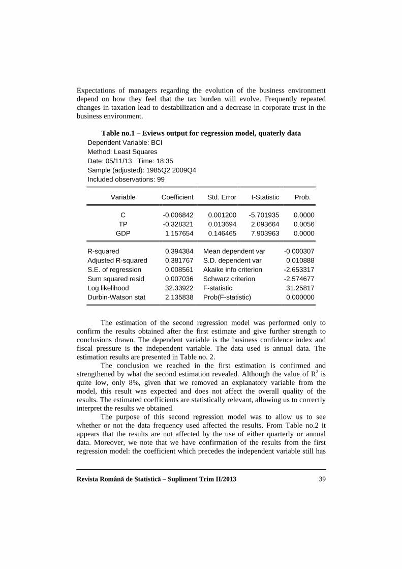
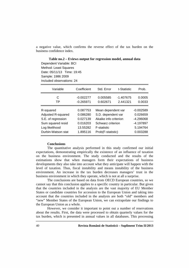
There are many factors that influence managers' confidence in the business environment. Of all these factors of influence, the impact of taxation on business performance is the subject of the present study. To analyze how taxation affects the business confidence index, we used data collected for OECD European countries in estimating two different regression models. Our results will show that managers take changes in taxation into account when they anticipate the evolution of the business environment.
Introduction Taxation is an area in continuous change and transformation that affects
many aspects of daily life, whether we are aware of its influence or not. The business environment, in turn, responds to tax changes continuously. This study aims to analyse the link between the business confidence index which represents managers’ view on the evolution of the business environment, and taxation, represented by the evolution of the tax burden as a percentage of total tax revenues in the gross domestic product.
Business stability is related to fiscal stability and our research aims to reveal these connections. Our study is organized into three parts. The first part concerns the existing state of current research on the problem that we analysed. The second part presents the methodology used in our study, and the last part presents the results obtained from the research conducted. Towards the end we have included conclusions and bibliography.
1. Literature Review
Revista Română de Statistică – Supliment Trim II/2013 36
Fiscal pressure has been a topic of interest to researchers for several decades, but always managed to remain a current issue. Donnahoe (1947) proposed a classification of the tax burden into three categories which he represented using a chart with straight lines and different slopes. He also proposed an interpretation of the tax burden as the ratio of a state's ability to generate taxes and the collection thereof. Browning (1978) studied tax burden and he demonstrated that indirect taxes tend to be progressive when examined in the context of a general equilibrium model in which transfers are an important source of income for the population. The study concludes that a system of regressive taxation can mean a reduced tax burden for the poorer taxpayers.
Lately, increasingly more studies have begun to focus on the index of business confidence. Collins (2001) examined the causal link between the index of business confidence and capital market development. For his study he used Granger causality and the conclusion reached was that the index of confidence in the business environment cannot be used to predict stock market trends, but developments in the capital market can be used to predict the index of business confidence.
But interest in the index of business confidence is older than that. For example, both Jacobs (1988) and Quinn (1989) have conducted studies which focused on the index of business confidence. Earlier still, Darling (1955) published a study on the statistical analysis of covariance between the index of business confidence and capital market prices.
Hohnischa, Pittnauerc, Solomond and Stauffere (2005) used data collected through surveys on businesses in Germany from 1960 onwards and proposed a stochastic model of the formation of individual expectations regarding business development in a particular industry sector. Taylor and McNabb (2007) analysed the possibility of using the index of confidence in the business environment as a tool for prediction and concluded that this index can be used to predict the downturns in the evolution of a particular sector.
Unfortunately, the existing literature makes very few references to studies linking taxation and the development of the business environment. Hence the innovative potential of the analysis we propose herein below.
2. Research Methodology The main variables used in our analysis are tax pressure and the business
confidence index calculated according to the OECD methodology. These are variables that particularly interest us, although the expectations of entrepreneurs regarding the evolution of the business environment obviously depend on many other factors besides tax developments.
To establish the indicator that we called tax burden we had several options available: total tax revenue ratio to GDP, the percentage of corporate tax revenues to GDP, the percentage of revenues from social contributions paid by the employer to GDP, the percentage of revenues from production related taxes to GDP and the
Revista Română de Statistică – Supliment Trim II/2013 37
percentage of revenues from customs duties to GDP. In order not to restrict in any way the relevance of the data used and because we thought that the first option of determining the tax burden includes virtually all the others, we decided to use fiscal pressure value determined as a percentage of total tax revenue to GDP. In our analysis we considered that the evolution of this variable from one time period to the next reflects the impact of the tax burden on business taxation.
The business confidence index is an indicator calculated on the basis of surveys for managers of enterprises operating in different fields. At EU level, this index is calculated separately for the main business sectors: industry, construction, retail and services. Moreover, an index is determined and allocated to the whole business environment, but it is computed only for the 17 Member States of the European Union that are also part of the Euro zone. This indicator can be seen in Chart no.1.
Our first observation is that the business confidence index is calculated on a monthly basis. It is based on business surveys containing questions managers answer. The answers are multiple-choice and of a qualitative nature, which makes the time spent completing the survey to be much lower compared to a survey that would require quantitative answers and would force the manager to constantly turn to the financial statements of the company for the necessary information to respond to the questions in the survey. Qualitative responses are converted into scores based on a well-established methodology and then contribute to the final score of the business confidence index.
The index of business confidence reflects managers’ perspective on the current situation of the company they lead in terms of performances but also their expectations for future developments. Thus, in our analysis, we found that this index represents the performance of firms operating in a particular geographical area.
Revista Română de Statistică – Supliment Trim II/2013 38
We included among the variables used the Gross Domestic Product, calculated in millions of U.S. dollars, because we thought it would be useful to compare the impact of the tax burden on business performance and impact of the GDP on the same dependent variable. The data used was collected for the OECD Europe zone, which means European countries that are also members of the OECD1. This geographical area is not equivalent to the Euro zone or the EU, but we considered that of all the alternatives available in the database of the OECD, data for this area was most relevant in order to reach a conclusion that would apply to the EU member states.
The time period considered is between 1985 and 2009, as more recent data than 2009 is not yet available on the OECD website. The data used is quarterly data for one of the regression models and annual data for the other regression model. Data for the business confidence index is monthly data, which was transformed into quarterly or annual data using a simple arithmetic mean. The source of data processed and subsequently used in our research is the OECD database, available online.
3. Results Our analysis is focused on the estimation of two linear regression models.
The first one has as dependent variable the index of business confidence and as dependent variables the GDP and the tax burden. The data used in the estimation is quarterly data for the period 1985-2009, modified to show changes in relative values for a certain period relative to the previous period, to ensure we used stationary time series. The estimation results are presented in Table no. 1.
The regression model may be considered valid despite the R2 value of only 39%. Given the nature of the variables used, we consider it an encouraging result which shows that nearly 40% of the index of confidence in the business environment can be explained by the evolution of the tax burden and the GDP. It would be unrealistic to expect a higher value of R2 given the multitude of factors that can influence managers' expectations about the evolution of the company they run, factors that were not included in our analysis. Regarding the coefficients that determine the independent variables and the free coefficient, the t-statistic tests as well as the F-statistic test and the probabilities attached to these tests show that these coefficients are statistically significant.
Thus, we can say that the tax burden inversely influences the evolution of corporate performance. An increase in the tax burden by one percentage point causes a decrease of the business confidence index by 0.32 percentage points.
1 The OECD Europe zone: Austria, Belgium, Czech Republic, Denmark, Estonia, Finland, France, Germany, Greece, Hungary, Ireland, Italy, Luxembourg, Netherlands, Norway, Poland, Portugal, Slovakia, Slovenia, Spain, Sweden, Switzerland, Turkey, United Kingdom
Revista Română de Statistică – Supliment Trim II/2013 39
Expectations of managers regarding the evolution of the business environment depend on how they feel that the tax burden will evolve. Frequently repeated changes in taxation lead to destabilization and a decrease in corporate trust in the business environment.
Table no.1 – Eviews output for regression model, quaterly data
Dependent Variable: BCI Method: Least Squares Date: 05/11/13 Time: 18:35 Sample (adjusted): 1985Q2 2009Q4 Included observations: 99
Variable Coefficient Std. Error t-Statistic Prob.
C -0.006842 0.001200 -5.701935 0.0000 TP -0.328321 0.013694 2.093664 0.0056
GDP 1.157654 0.146465 7.903963 0.0000
R-squared 0.394384 Mean dependent var -0.000307 Adjusted R-squared 0.381767 S.D. dependent var 0.010888 S.E. of regression 0.008561 Akaike info criterion -2.653317 Sum squared resid 0.007036 Schwarz criterion -2.574677 Log likelihood 32.33922 F-statistic 31.25817 Durbin-Watson stat 2.135838 Prob(F-statistic) 0.000000
The estimation of the second regression model was performed only to
confirm the results obtained after the first estimate and give further strength to conclusions drawn. The dependent variable is the business confidence index and fiscal pressure is the independent variable. The data used is annual data. The estimation results are presented in Table no. 2.
The conclusion we reached in the first estimation is confirmed and strengthened by what the second estimation revealed. Although the value of R2 is quite low, only 8%, given that we removed an explanatory variable from the model, this result was expected and does not affect the overall quality of the results. The estimated coefficients are statistically relevant, allowing us to correctly interpret the results we obtained.
The purpose of this second regression model was to allow us to see whether or not the data frequency used affected the results. From Table no.2 it appears that the results are not affected by the use of either quarterly or annual data. Moreover, we note that we have confirmation of the results from the first regression model: the coefficient which precedes the independent variable still has
Revista Română de Statistică – Supliment Trim II/2013 40
a negative value, which confirms the reverse effect of the tax burden on the business confidence index.
Table no.2 – Eviews output for regression model, annual data
Dependent Variable: BCI Method: Least Squares Date: 05/11/13 Time: 19:45 Sample: 1986 2009 Included observations: 24
Variable Coefficient Std. Error t-Statistic Prob.
C -0.002277 0.005585 -1.407675 0.0005 TP -0.265971 0.602671 2.441321 0.0033
R-squared 0.087753 Mean dependent var -0.002589 Adjusted R-squared 0.086280 S.D. dependent var 0.026659 S.E. of regression 0.027139 Akaike info criterion -4.296068 Sum squared resid 0.016203 Schwarz criterion -4.197897 Log likelihood 13.55282 F-statistic 5.194764 Durbin-Watson stat 1.895116 Prob(F-statistic) 0.003288
Conclusions The quantitative analysis performed in this study confirmed our initial
expectations, demonstrating empirically the existence of an influence of taxation on the business environment. The study conducted and the results of the estimations show that when managers form their expectations of business developments they also take into account what they anticipate will happen with the level of taxation. Thus, fiscal instability and means instability of the business environment. An increase in the tax burden decreases managers’ trust in the business environment in which they operate, which is not at all a surprise.
The conclusions are based on data from OECD European countries, so we cannot say that this conclusion applies to a specific country in particular. But given that the countries included in the analysis are the vast majority of EU Member States or candidate countries for accession to the European Union and taking into account that the countries included in the analysis are both “old” members and “new” Member States of the European Union, we can extrapolate our findings to the European Union as a whole.
However, we consider it important to point out a number of reservations about the results. First, the data were processed to obtain quarterly values for the tax burden, which is presented in annual values in all databases. This processing
Revista Română de Statistică – Supliment Trim II/2013 41
could affect the quality of information contained in the observations used for this variable. Secondly, for the second regression we could only get data for 24 observations, which could affect the statistical significance of the results. Finally, the low value of the regression coefficient R2 for both models, although justifiable, makes us believe that we should take the study further by introducing several more explanatory variables in the regression model. References Browning, E. - The Burden of Taxation, The Journal of Political Economy,1978, 86
(4), pp. 649-671 Collins, D. – The Relationship between Business Confidence Surveys and Stock
Market Performance, Investment Analysts Journal, 2001, 54, pp. 9-17 Darling, P.G. - A Surrogative Measure of Business Confidence and Its Relation to
Stock Prices, The Journal of Finance, 1955, 10, pp. 442–458 Dickey, D.A. & Fuller, W.A. – Distribution of the estimators for autoregressive
time series with a unit root, Journal of the American Statistical Association, 1979, 74, pp.427-431
Donnahoe, A. - Measuring State Tax Burden, The Journal of Political Economy, 1947, 55 (3), pp. 234-244
Heye, C. - Labour Market Tightness and Business Confidence: An International Comparison, Politics & Society, 1993, 21, pp. 169-193
Hohnischa, M. Pittnauerc, S. Solomond, S. & Stauffere, D. - Socioeconomic interaction and swings in business confidence indicators, Physica A: Statistical Mechanics and its Applications, 2005, 345 (3–4), pp. 646–656
Keho, Y. - Budget balance through revenue or spending adjustments? An econometric analysis of the Ivorian budgetary process, 1960 – 2005, Journal of Economics and International Finance, 2010, 2(1), pp. 001-011
OECD - Business Tendency Surveys: A Handbook, Statistics Directorate, Paris, 2003
OECD - Introducing OECD Standardised Business and Consumer Confidence Indicators and Zone Aggregates, Main Economic Indicators, 2006
Quinn, D.P. - Corporate Taxation and Corporate Economic Power: Testing Class-Power and Business-Confidence Models, American Journal of Sociology, 1989, 94 (6), pp. 1419-1426
Taylor, K. & McNabb, R. - Business Cycles and the Role of Confidence: Evidence for Europe, Oxford Bulletin of Economics and Statistics, 2007, 69, pp. 185–208
Revista Română de Statistică – Supliment Trim II/2013 42
Reforming the Eurozone
Prof. Radu Titus MARINESCU, PhD
„Artifex” University of Bucharest Prof. Constantin ANGHELACHE, PhD
„Artifex” University of Bucharest / Academy of Economic Studies, Bucharest
Valentin BICHIR, PhD Student Academy of Economic Studies, Bucharest
Alex BODISLAV, PhD Student Academy of Economic Studies, Bucharest
Abstract In the heat of the debt crisis, German Chancellor Angela Merkel
made an admission that clarified for many the stark choices facing Europe: rolling government debt too far into the future was no longer an option for Germany because there was no guarantee the country’s aging population could cover the bills once they came due. in a nutshell, Merkel illustrated the problems facing the European Union’s “social market economy.” lavish retirement and welfare benefits begun during the vibrant years of the post-world war II boom may not be affordable in an era of declining population, slower economic growth and waning competitiveness. Key words: government, investor, fiscal union, budget, sovereignty
JEL Classification: N10, N14
“The new German problem is that the future of the Eurozone and of Europe rests on the dominant German economy, but the long-term prospects of German demographics are daunting,” a United Press International article said in 2011. “After three decades of dwindling birth rates there will simply not be enough Germans of working age to sustain the burden.” This analysis suggests that even if the Eurozone emerges from the crisis that began in Greece and bled into countries such as Italy, the respite may only be temporary. To break the impasse, Europeans have floated possible longer-term solutions to the euro predicament, none of which will be easy to achieve in an EU built upon the principle of unanimous decision-making among its 27 members. Many EU leaders see the eurozone evolving into a fiscal union in which richer members such as Germany help pay the debts of other members, in some cases through “eurobonds” issued jointly by the EU. That would require structural reform to relatively unproductive EU economies that have used the euro to finance unsustainable spending. Once nations commit to spending
Revista Română de Statistică – Supliment Trim II/2013 43
discipline, economists view economic growth as the ideal way to shrink debt relative to the size of the economy. In Europe’s case, however, such growth could be stymied by low birthrates and growing intolerance for mass immigration.
“Growth is undoubtedly the best way to get out of the debt trap. After World War II, the American economy grew at a faster rate than the national debt. As a result, the debt ratio was automatically reduced,” Der Spiegel wrote in January 2012. “Nowadays, however, an aging and shrinking population makes it far more difficult to increase economic output. This means that slow-growing countries like Japan or Germany can hardly serve as the reliable borrowers of tomorrow. Rising economies like China, India, Indonesia, the Philippines or Vietnam offer more security.” Hurdles to fiscal union The origin of the European debt crisis was the 2008 revelation that Greece could no longer meet its bond payments, money it had borrowed from domestic and international investors to finance government spending. Greece has since benefited from an EU bailout fund strengthened with hundreds of billions of euros from donors such as Germany. Greek leaders have also negotiated with bondholders to cancel or refinance most of the country’s outstanding debt, which exceeds the country’s gross domestic product. Though Greece’s future as a member of the eurozone remains in doubt, a potentially greater danger is that the financial contagion could spread to the much larger economies of Italy and Spain. Even France, once perceived as an impeccable investment for creditors, had its bond rating downgraded in early 2012, suggesting the country will eventually have to pay higher interest rates to borrow money. Many EU members have responded by calling for greater fiscal integration of a continent where national parliaments still control almost all budgeting. Despite pressure from France, Germany has rejected the concept of debt pooling until its taxpayers are assured they won’t be picking up the tab for prodigal spending in the countries of the Mediterranean. But the price of such reassurance may be too high: EU members would have to cede budgetary control, a critical part of national sovereignty, to Brussels. Achieving unanimity on that point among 27 different national electorates (17 electorates if the changes were confined to countries using the euro) could be difficult.
“Shared liability is something we will only be able to contemplate once the EU has achieved much greater integration. It will not do as a means to resolve this crisis,” Merkel explained in an interview with theGuardian in January 2012. “That greater integration would involve the European court of justice enforcing controls for national budgets, for example, and much more besides. If we at some point have harmonized our financial and budgetary policy, that will be the time to try and find other forms of cooperation and shared liability.” Growth through reform When facing similar financial crunches in the past couple of decades, countries such as Sweden and Finland reacted by deregulating and restructuring their economies, which they believed had grown too rigid and uncompetitive. Sweden experimented successfully with deregulation of its retail sector that
Revista Română de Statistică – Supliment Trim II/2013 44
allowed companies such as furniture seller IKEA to thrive. It partially privatized its government-guaranteed pension system on a model provided by Chile. As a result, the country outperformed most of the continent in terms of productivity and investment, and has weathered the recent crisis better than most.
“Europe’s governments have been remarkably timid, compared with the Nordics, in exploiting another avenue to growth – structural reform,” the Economist noted in January 2012. “… it is in Europe where the potential gains from structural reforms are greatest and where the policy focus has nonetheless been overwhelmingly on austerity.”
As the recent crisis took hold, Spain and Italy have both promised to loosen labor rules that have locked older workers into jobs and deprived young aspirants of access to those same fields. Stories proliferate about trucking licenses in Greece passing from generation to generation like treasured inheritances unavailable to outsiders. Italian labor rules fill 2,700 pages and are so murky that businesses can’t fire incompetent workers without stiff penalties or labor strife, Bloomberg Businessweek wrote in late 2011. The country ranks near the bottom of the world in labor market efficiency.“ Italy’s economy can no longer afford the generous benefits it showered on its workers in the 1960s, when the country grew 5 percent to 6 percent a year,” the magazine noted. “Measures put in place years ago to protect workers aren’t just slowing down the economy now, they’re perversely hurting the very workers they’re meant to protect.” Stopping population decline Few doubt anymore that European infertility correlates to the euro crisis. In a January 2012 article, Der Spiegel suggested governments re-evaluate government debt in light of demographic change. Sovereign debt was once deemed necessary for war fighting and investment in projects such as dams, bridges and airports. But these days almost every finance ministry piles debt upon debt simply to pay for ongoing expenses such as government salaries and pensions. Such a bargain is workable if a country’s working age population rises compared with the number of retirees. But that’s not the case in almost all of Europe. Fewer workers will be available to be taxed to finance the retirements of a growing pool of elderly pensioners. Long-term bondholders asked to wait 30 years to redeem their investments are worried about the EU’s financial viability by the time 2042 rolls around. Many of the problems revealed during the euro crisis were outlined in “Project Europe 2030: Challenges and Opportunities,” a report produced for the European Commission in 2010. The 46-page document starkly laid out problems needing the coordinated attention of EU member states lest they slide into irrelevance on the world stage. At the current average birthrate of about 1.3 children per woman — the replacement rate is nearly 2.1 children per woman — the EU would face massive worker shortages requiring tens of millions of immigrants to fill.
Revista Română de Statistică – Supliment Trim II/2013 45
“Too often immigration is perceived as a burden to be shouldered rather than an opportunity to be seized. Europe has much to learn in this regard from Australia, Canada and the United States, with which it is in direct competition for talented and skilled immigrants,” the report said. “yet Europe will only become an attractive destination for skilled immigrants if the latter feel accepted, have full access to formal labour markets and the possibility to set up their own businesses.” The opening of EU labor markets in 2011 to recently admitted member states such as Poland and the Czech Republic promises to help improve the situation. But EU officials believe the continent will need to look farther abroad to fill its need for scientists, researchers and doctors. A “blue card” program giving preferential immigration treatment to highly educated arrivals from Asia, Africa and North America would help. “Project Europe” says as much. Attempts by governments such as Germany’s to encourage families to breed have largely failed, stymied by changing cultural attitudes that government bureaucrats struggle to recognize. Germany has already spent 15 billion euros ($21 billion) on Elterngeld to subsidize child rearing. “But no matter how much money the state throws at the problem, it won’t go away,” Der Spiegel concluded in August 2011. Reasons for hope The EU remains the world’s largest economic bloc packed with 500 million citizens living in democracy and freedom. The continent will eventually emerge from its debt crisis, either with a more compact eurozone or a recommitment to stronger fiscal union, but the bigger challenge will be declining European competitiveness and addiction to unaffordable government spending. What EU leader wants to preside over a shrinking, less influential Europe lacking even the means to defend itself? As Italian Prime Minister Mario Monti phrased it in January 2012: “Overcoming the economic, financial and social crisis that is gnawing at Europe depends on structural reforms that are in the hands of, and in the decision-making capacity of, the member states.” Transparency Counters Corruption
The open Government Partnership improves national accountability In September 2011, the United Nations introduced the open government
partnership (OGP), an ambitious multinational initiative that aims to disclose government information to citizens. Such transparency can uncover and dissuade corruption, bolster accountability among government officials and empower citizens to team up with their government to promote honest administration. The partnership calls for governments to post budgets and financial documents online, as well as disclose the assets of public officials, and encourages citizen whistleblowers to report irregularities. Serving as a network of support, the initiative provides a framework for countries to start their own domestic open government policies – a task some states find too daunting to undertake alone. The partnership has already garnered commitments from 42 nations and many others are earmarked for membership. Supporters insist the OGP represents a significant step toward global transparency over national accountability
Revista Română de Statistică – Supliment Trim II/2013 46
Openness is good for the economy
The program’s core function is to educate and inform citizens. U.S. Secretary of State Hillary Clinton says there is an “undeniable connection” between how governments function and whether their people flourish, a July 2011 Voice of America article reported. Additionally, open government is helpful to economic growth. Entrepreneurs are attracted to countries that fight corruption and promote transparent government. Openness is beneficial not only for “good government” but for sustained economic growth. As government budgets tighten, transparency can encourage trade and outside investment in a state. How it works Armenia, Bulgaria, Georgia, Greece, Romania and Turkey are among the numerous countries participating in the OGP. The program starts with governments developing and implementing country-specific reform plans and communicates concrete commitments surrounding five “grand challenges”: improving government services, increasing public integrity, managing public resources more effectively, increasing corporate accountability and creating safer communities. After a year of implementation, each government submits a progress report, and each country is evaluated by well-respected local governance experts that will independently assess each country’s progress. Brazilian Foreign Minister Antonio Patriota assured prospective OGP participants in June 2011 that reviews will not include “quality labels” or “rankings” and will be conducted in a “technical, neutral and no adversarial manner.” Nation eligibility list Twenty-nine additional countries are eligible for membership. An independent group of experts have evaluated and chosen countries by scoring them on fiscal transparency, freedom of information, public figure asset disclosure and engagement of citizens. They must score at least 12 out of 16 to qualify. Italy, Norway, Romania, Sweden, the United Kingdom and the United States scored among the highest; Armenia, Israel, Panama and Paraguay scored among the lowest, but still made the list. Some, however, have questioned the list and its accuracy. Notably, Russia and Pakistan, nations that don’t always have a reputation for transparency, are eligible, according to the OGP. And surprisingly, Georgia scored higher than the more developed democracies of Denmark, Estonia and Iceland. Placing countries on this list can provide an incentive to strive for openness and inspire reform. Georgia is a good example of this, as it is taking steps toward transparency, but organizers say the nation still has room to improve.
A May 2011 Transparency International (TI) assessment report suggests that countries in the South Caucasus need to strengthen anti-corruption policies. “They should take note that citizens are no longer willing to be passive spectators; they are increasingly showing that they are tired of mismanagement and corruption,” said Jana Mittermaier, head of TI’s Liaison Office to the European Union. The European nations of Bosnia and Herzegovina, Finland, France,
Revista Română de Statistică – Supliment Trim II/2013 47
Germany, Hungary, Iceland and Poland stand to benefit from joining as well, but had not as of early 2012.
A central part of the plan is collaboration with nongovernmental organizations (NGOs). One country in particular is making headway on this front. The Slovakian organization Fair Play Alliance has teamed up with the Slovakian government to reveal the names of those doing business with the government, supplying citizens with information to probe deeper into those relationships. NGOs provide opportunities to complement ongoing reform and monitor implementation, while TI, a nonpartisan organization fighting corruption worldwide, publishes a well-regarded list on government openness that addresses the scale and challenges of government corruption. Founding partners The partnership is currently led by the U.S. and Brazil and is supported by six other founding partner nations: Indonesia, Mexico, Norway, the Philippines, South Africa and the UK. Leadership of the group will rotate annually among founding partners, with the UK co-chairing the OGP in 2012. Brazil has used the leadership opportunity to establish a “transparency portal” that reports government spending information and fund transfers, and, despite challenges, established a Freedom of Information Act through which citizens can request previously hidden information. The U.S. has joined the Extractive Industries Transparency Initiative, a partnership that requires governments, and oil, gas and mining companies to disclose financial transactions among themselves. The U.S. also established an online petition platform offering Americans a vehicle for communicating with the government. Some open government activists question whether Brazil deserves to be a co-leader. They criticize Brazil for failing to have a Freedom of Information Act at the time of admittance – a membership requirement some activists consider fundamental. Establishing the act was stalled by controversy over the opening of past military documents, but in late 2011 the process was completed. Speculation remains, however, how it will pan out. “It now remains to see how the law will be actually implemented, and if access to public information will become an effective tangible right for most citizens,” said Brazilian scholar and commentator Ronaldo Lemos In late 2011 in a blog hosted by Princeton’s Center for Information Technology Policy. Additional objections include accusations of corruption among government officials. “Joining the U.S. in shepherding the partnership to fruition was Brazil, which has seen five cabinet-level officials leave government in the last nine months amid corruption scandals,” the Wall Street Journal reported in September 2011. More transparency needed Deeper reform is needed for transparency to have a more striking impact. “Publishing official statistics and general budget data online can be a first step, but one ought not declare ‘premature victory’ after tackling such generic ‘low hanging fruits,’ ” the U.S.-based Brookings Institute said. Brookings praised the benefits of “more politically difficult reforms, such as transparency in the drafting of laws and
Revista Română de Statistică – Supliment Trim II/2013 48
in policymaking, campaign finance, lobbying, the disclosure of officials’ assets, and fully disclosing which powerful private sector and media executives the leaders of government meet regularly with.”
The UK’s efforts, for example, encompass openness of data and statistics, including medical information. Publishing health care statistics is one example of how exposure to information can save lives. At the commencement of the partnership in 2011, a UK representative pointed out how publishing surgery mortality rates among surgeons exposed remarkable differences in physician quality. Some doctors were put out of business. By publishing data, bad practices were rejected and good practices multiplied. The UK government said transparency helped the country drop surgical mortality rates by as much as 22 percent. Technological transformation Citizens are increasingly demanding greater democracy through technology. Demonstrated by the North African revolutions, citizens using social media can heavily influence government. Technology played an invaluable role in empowering citizens to demand freedom against seemingly insurmountable odds and helped shame governments into addressing corruption. It is yet to be seen whether technology will prove equally as effective in constructing fully open societies. “When a government hides its work from public view, hands out jobs and money to political cronies, administers unequal justice, looks away as corrupt bureaucrats and businessmen enrich themselves at the people’s expense, that government is failing its citizens,” Secretary of State Clinton said. Establishing government transparency “can be a lonely, sometimes even dangerous task. But through this partnership, we hope to change that,” she added. Multinational collaboration in the OGP strives to set standards for transparency and is a solid starting point in countering corruption and empowering citizens to hold governments accountable. References Bochko V. The formation of intelligence-innovations territories, în: Alexander
Tatarkin & Antonio Sanchez (ed.) Economy of Russia and Europe: problems and cooperation prospects, 2009, p: 98-109
Edgar B., Scenario Planning as a Tool to Promote Innovation in Regional Development Context, European Regional Science Association în ERSA conference papers, 2011.
Frăţilă L. et al., The Business Intelligence and the Better Decisions in Management, Review of International Comparative Management, Volume 12 2011, P: 332-338.
Iordache E., Voiculeţ A.V., Romania’s competitive advantage within the European Union area, University Library of Munich, Germany in MPRA Paper, 2007.
Revista Română de Statistică – Supliment Trim II/2013 49
The Relevance of the Rural – Urban Covergence Based on a New Method of Price Shears’ in
Romanian Economy
Assoc. prof. Gheorghe SĂVOIU, PhD University of Pitesti
Prof. Laurenţiu TĂCHICIU, PhD Academy of Economic Studies, Bucharest
Prof. Vasile DINU, PhD
Academy of Economic Studies, Bucharest Abstract The authors of this paper had tried to answer to some major
questions about the importance and the consequences of the contemporary prices shear in the Romaniana economy. How important could be the consumer price index (CPI) in today’s Romanian market economy? Could the current prices shear revealed by the structural inflation indexes be a real instrument for a rural and urban ceconomic convergence in Romania? The method of price shears used for the first time in contemporary Romanian economy, based on its new statistical instrument and indices for inflation’s evaluation allows a significant turning to account of the inflation rural / urban disparities, whose statistical and economic consequences are very important today. The methodology of this paper is predominantly statistical, highlighting the qualities of the current Romanian interpreter index of consumer prices, focusing on the strengths of its practical utility and specificity.
Key words: consumer price index (CPI) the goods – services price shears, inflation, interpreter index, matrix of correlations.
JEL Classification: O18, E31
The tradition of price shears, maintained in the national economy to the detriment of the countryside, is recorded (Madgearu, 1940, p. 61) and evaluated between 1929 and 1938, fluctuating between a minimum of 23.35 and 36.2% (Georgescu-Roegen, 1943, p 81). What this article proposes is a product – service price shears based on a double reality, the domination of the primary sector (agriculture, forestry and food industry) in the Romanian rural territory and the
Revista Română de Statistică – Supliment Trim II/2013 50
almost exclusively presence of the tertiary sector and services in urban areas, which is essentially part of the same traditional line.
The authors of this paper had tried to answer to some major questions about the importance and the consequences of the contemporary prices shear in the Romaniana economy. How important and relevant could be the consumer price index (CPI) in today’s Romanian market economy? Could be the current prices shear a real and a pragmatical instrument revealed by the structural inflation indexes for a rural and urban ceconomic convergence in Romania?
The method of price shears allows a significant turning to account of the inflation index for services, whose statistical and economic impact remains very important. The price shears in commerce-related and marketing activities, determined especially in foreign trade (Săvoiu and Dinu, 2012; Săvoiu, Dinu and Tăchiciu, 2012) is calculated only if the index of the net exchange ratio is smaller than 1 (IRSN < 1 or 100%). Price shears in foreign trade expresses the percentage loss on an economy, an area or a sector or a particular type of activity, which is recorded by foreign trade due to the fact that export prices fail to keep pace with the prices of imports. GENERAL PRICE SHEARS or FTPS = (1-IRSN) × 100 (1)
In terms of territory, it becomes a relationship between export prices and
tariffs and their import counterparts, in relation to the respective territory. What can be easily found is that there is a certatin tradition of persistence of an urban – rural price shears in the Romanian economy. A rural household price shears actually reflects their effort, which is much higher as a result of the territorial distribution of inflation; their incomes, very small as they are, experience an extra loss in their substance, approximately 27% more than those in urban areas, due to the much sharper rise in non-food prices.
On the whole of the Romanian economy, between 1990 and 2012, a general price shears can be determined according to the relation GENERAL PRICE SHEARS or FTPS = (1-INB) × 100 = (1-UVIX : UVIM) × 100 (2) or translated within the context of foodstuff inflation (CPIfood) and services (CPIservices) becomes: GENERAL PRICE SHEARS or FTPS = (1-CPIfood : CPIservices) × 100 (3) the result of which is (1 – 276167.46 : 664251.64) : 100 = 58,4%, which indicates a loss or an unpaid transfer from the primary sector, typical of rural areas, to the
Revista Română de Statistică – Supliment Trim II/2013 51
tertiary sector, characteristic of urban areas, of about 6/10 over the period under analysis.
Table no.1. The annual price shears product - service tariff, in Romania,
between 1991 and 2012 (%)
CPI food product
CPI Services
Product – services tariff price shears
Year1991/1990 286.2 235.7 No service tariff price shears Year1992/1991 336.6 280.4 No service tariff price shears Anul1993/1992 348.9 340.3 No service tariff price shears Year1994/1993 236.2 250.8 5.82 Year1995/1994 131.9 142.7 7.57 Year1996/1995 136.4 146.9 7.15 Year1997/1996 251.4 276.5 9.08 Year1998/1997 148.4 192.1 22.75 Year1999/1998 127.9 184 30.49 Year2000/1999 143.7 153.9 6.63 Year2001/2000 135.7 135.4 No service tariff price shears Year2002/2001 118.3 126.8 6.70 Year2003/2002 114.7 114.8 0.09 Year2004/2003 109.5 114.7 4.53 Year2005/2004 106.1 110.5 3.98 Year2006/2005 103.84 108.2 4.03 Year2007/2006 103.89 106.63 2.57 Year2008/2007 109.22 108.57 No service tariff price shears Year2009/2008 103.25 108.97 5.25 Year2010/2009 102.33 104.78 2.34 Year2011/2010 106.02 104.45 No service tariff price shears Year2012/2011 101.89 105.07 3.18 Source: http://www.insse.ro/
The detailed method of price shears evaluation is summarized in Table 1, where there are the signs of inflation for foodstuffs and services, as well as the product – service tariff price shears in Romania, between 1991 and 2012. The next table (2) presents an image of the major rates from Romanian economy including the product services tariff price shears, with the intention of underlying the existence of the correlation between the economic growth rate and the product services tariff price shears, a correlation that must be tested.
Revista Română de Statistică – Supliment Trim II/2013 52
Table no.2. The annual price shears product - service tariff and the growth rate, in Romania, between 1991 and 2012
Table no.3. The correlation matrix between the rates of economic growth, general inflation and price shears product - service tariff in Romania, between
C 5.222714 3.170126 1.647478 0.1151 SER03 -0.858708 0.344479 -2.492772 0.0216
R-squared 0.237046 Mean dependent var 0.454545 Adjusted R-squared 0.198899 S.D. dependent var 13.24796 S.E. of regression 11.85748 Akaike info criterion 7.870304 Sum squared resid 2811.999 Schwarz criterion 7.969489 Log likelihood -84.57334 F-statistic 6.213914 Durbin-Watson stat 1.995299 Prob(F-statistic) 0.021564
Software used: Eviews and a multifactorial model of the real GDP in Romania (SER01)
explained by the general inflation or the rate of PCI(SER02) and the price shears product - service tariff (SER03)
Table no. 5
Dependent Variable: SER01 Method: Least Squares 1991 2012 Variable Coefficient Std. Error t-Statistic Prob. C 9.044824 3.627439 2.493446 0.0220 SER02 -0.060553 0.032516 -1.862232 0.0781 SER03 -0.910991 0.326220 -2.792566 0.0116 R-squared 0.354808 Mean dependent var 0.454545 Adjusted R-squared 0.286893 S.D. dependent var 13.24796 S.E. of regression 11.18732 Akaike info criterion 7.793564 Sum squared resid 2377.968 Schwarz criterion 7.942342 Log likelihood -82.72920 F-statistic 5.224296 Durbin-Watson stat 2.477964 Prob(F-statistic) 0.015561
Software used: Eviews The last model could constitute a good option for a new kind of analysis
of the rural –urban convergence in Romania (based on the data presented in Table 4 and 5 (where the rate of the price shears product - service appears as exogenous variables with a reasonable determination (the value of R being 0.60638).
Conclusions The method of price shears product - service tariff can be optimized by
calculating the effect, in absolute terms, of the deterioration of the net exchange ratio (∆NBR), by assessing, in national currency, the impact of the existence of the price shears. The model of economic growth rate as an endogenous factor explained by the general PCI and price shears product - service tariff in Romania
Revista Română de Statistică – Supliment Trim II/2013 54
could be a good start option for a new method of analysis of the rural – urban convergence in our economy.
References Georgescu-Roegen, N. (1997), Romanian Economy, Bucharest, Editia I, 1939-
1940, in Romanian Encyclopedia, Expert publishing House, reeditată. Madgearu, V. (1995), Evoluţia economiei romănesti după războiul mondial, Ediţia
I 1940, Ed. Stiinţifică, Bucuresti, reeditată. Săvoiu, G. (2001), The Price Universe and Interpret Index, Pitesti, Economical
Independence Publishing House. Săvoiu, G. et al. (2007), A Romanian Centennial Price Index, Progresses in
Economic Decision Theory in Risk and Incertitude Conditions. Fuzzy in Economics Romanian Academia International Conference, Jassy. Performantica Publishing House,Vol. II, 2007, pp.171-185.
Săvoiu, G., Dinu, V. (2012), Solutions for the Statistical Analysis of the Economic Phenomena Described as Opposed, Partially of Entirely Compensated Fluxes, A Case Study on the Exports and Imports of Romania and the Baltic States. Transformations in Business & Economics, Vol 11, 1 (25), pp. 54-71
Săvoiu, G., Vasile, D., Tăchiciu, L., (2012), Romania Foreign Trade in Global Recession, Revealed by the Extended Method of Exchange Rate Indicators, Amfiteatru Economic, XIV(31), pp.173-194.
Revista Română de Statistică – Supliment Trim II/2013 55
The Features of the Chronological Series of Statistical Indices
Prof. Constantin ANGHELACHE PhD „Artifex” University of Bucharest/
Academy of Economic Studies of Bucharest Prof. Vergil VOINEAGU PhD
Academy of Economic Studies of Bucharest Mihai GHEORGHE PhD
National Institute of Statistics Ec. Cristina SACALĂ
National Institute of Statistics Ec. Ionuţ NEGOIŢĂ
Manager Ec. Alexandru URSACHE
Abstract The characterization of the evolution over a past period (ex-post) of
the prices for consumption goods and services acquired on the market implies the construction and the analysis of the specific chronological series. These series are built up for both absolute and relatives indicator, mainly for indices.
When building up the series of the individual indices of prices there are not particular difficulties to expect; the only aspect which must be analyzed with discernment and, consequently, to be decided, is regarding the choice of the reporting basis, which can be fix or mobile (chained). In the case of the group series, the particular issue to face is given by the weighting system to consider, since it synthetizes the propensity for consumption of a period of time and this one is variable enough and has an impact of the index size. According to the reporting basis, the indices series of an ex-post period T;0 , is synthetically showed in the following matrix. This matrix gives us a complete image on the prices of the consumption goods and services of the population, implicitly on the forms in which the inflation is showing to the consumer.
Revista Română de Statistică – Supliment Trim II/2013 56
Out of the submitted matrix it is noticeable and can be analyzed:
− On the lines, there are the possible series of indices with fix base – the fix base being any period out of the analyzed time horizon
T;0 ; − On the diagonal there are the possible series of indices with mobile
base on each sub-period of the time horizon T;0 ; − On the column there are all the series of indices through which any
period Tt ;0∈ is compared as against all the previous periods. Between the indices shown by the series of the matrix there is the
following relation of system:
− 0/
11/ T
T
ttt II =∏
=−
- for each series of the matrix (1)
− 1/
0/1
0/−
−
= ttt
t III
- for each Tt ;0∈ (2) Depending on the weights used for building up the indices, in a series of
prices indices we can theoretically meet: − Indices with constant weights, when for the entire series the same
weights are utilized; − Indices with variable weights, when the weight changes every time
the reporting base is changed. By combining these variants, we can build up series of group indices with fix base and constant or variable weights and group indices with mobile base and constant or variable weights. Thus:
− Group indices with fix base and constant weights – taken from the base period. By developing the relation
Revista Română de Statistică – Supliment Trim II/2013 57
∑
∑
=
== N
iii
N
iiit
pt
qp
qpI
100
10
0/ , where Tt ;1= , Ni ;1= - expenses typology (3),
We get the corresponding series of indices:
Tt
N
iii
N
iiit
pt
qp
qpI
,1100
10
0/
==
=
⎪⎭
⎪⎬
⎫
⎪⎩
⎪⎨
⎧
=∑
∑ (4).
Similarly, we can get the series of indices for the variable iq , starting from the development of the relation:
∑
∑
=
== N
iii
N
iiti
qt
qp
qpI
100
10
0/ , where Tt ;1= (5)
namely
Tt
N
iii
N
iiti
qt
qp
qpI
,1100
10
0/
==
=
⎪⎭
⎪⎬
⎫
⎪⎩
⎪⎨
⎧
=∑
∑ (6)
− Group indices with chained base and constant weights. For the
variable ip the series of indices are resulting out of the development of the following relation:
∑
∑
=−
=− = N
iiit
N
iiit
ptt
qp
qpI
101
10
1/ , where Tt ;1= (7),
If the weights are taken from the base period and
∑
∑
=−
=− = N
iitit
N
iitit
ptt
qp
qpI
11
11/ , where Tt ;1= (8),
if the weights are taken from the current period. The out coming series of indices are the following:
Revista Română de Statistică – Supliment Trim II/2013 58
Tt
N
iiit
N
iiit
ptt
qp
qpI
,1101
10
1/
==−
=−
⎪⎭
⎪⎬
⎫
⎪⎩
⎪⎨
⎧
=∑
∑ (9)
şi
Tt
N
iitit
N
iitit
ptt
qp
qpI
,111
11/
==−
=−
⎪⎭
⎪⎬
⎫
⎪⎩
⎪⎨
⎧
=∑
∑ (10)
Between the elements of the two series (9) and (10) there are system relations, namely:
∑
∑∏
∑
∑∏
=−
=
=
=−
=
=− == N
iiit
N
iiiTT
tN
iiit
N
iiitT
t
ptt
qp
qp
qp
qpI
101
10
1
101
10
11/ , where Tt ;1= (11)
∑
∑∏
∑
∑∏
=−
=
=
=−
=
=− == N
iiTit
N
iiTiTT
tN
iitit
N
iititT
t
ptt
qp
qp
qp
qpI
11
1
1
11
1
11/ , where Tt ;1= (12)
For the variable iq , the series are obtained by developing the relations:
∑
∑
=−
=− = N
iiti
N
iiti
qtt
qp
qpI
110
10
1/ , where Tt ;1= (13),
If the weights are taken from the base period and
∑
∑
=−
=− = N
iitit
N
iitit
qtt
qp
qpI
11
11/ , where Tt ;1= (14),
If the weights are taken from the current period The resulting series of indices are the following:
Tt
N
iiti
N
iiti
qtt
qp
qpI
,1110
10
1/
==−
=−
⎪⎭
⎪⎬
⎫
⎪⎩
⎪⎨
⎧
=∑
∑ (15) and
Revista Română de Statistică – Supliment Trim II/2013 59
Tt
N
iitit
N
iitit
ptt
qp
qpI
,111
11/
==−
=−
⎪⎭
⎪⎬
⎫
⎪⎩
⎪⎨
⎧
=∑
∑ (16)
Between the elements of the two series (15) and (16) there is a system relation, namely:
∑
∑∏
∑
∑∏
=
=
=
=−
=
=− == N
iii
N
iiTiT
tN
iiti
N
iitiT
t
qtt
qp
qp
qp
qpI
100
10
1
110
10
11/ , where Tt ;1= (17)
∑
∑∏
∑
∑∏
=
=
=
=−
=
=− == N
iiiT
N
iiTiTT
tN
iitit
N
iititT
t
qtt
qp
qp
qp
qpI
10
1
1
11
1
11/ , where Tt ;1= (18)
− Indices with mobile base and variable weights For both variable ip and iq we can build up indices with variable weights
taken from the base period and from the currents periods. The general relations from which the series of indices result are the following:
∑
∑
=−−
=−
− = N
iitit
N
iitit
ptt
qp
qpI
111
11
1/ , where Tt ;1= (19)
∑
∑
=−−
=−
− = N
iitit
N
iitit
qtt
qp
qpI
111
11
1/ , where Tt ;1= (20),
And the corresponding series are:
Tt
N
iitit
N
iitit
ptt
qp
qpI
,1111
11
1/
==−−
=−
−⎪⎭
⎪⎬
⎫
⎪⎩
⎪⎨
⎧
=∑
∑ (21) şi
Tt
N
iitit
N
iitit
qtt
qp
qpI
,1111
11
1/
==−−
=−
−⎪⎭
⎪⎬
⎫
⎪⎩
⎪⎨
⎧
=∑
∑ (22)
If weights from the current period are utilized, the relations are:
Revista Română de Statistică – Supliment Trim II/2013 60
∑
∑
=−
=− = N
iitit
N
iitit
ptt
qp
qpI
11
11/ , where Tt ;1= (23)
∑
∑
=−
=− = N
iitit
N
iitit
qtt
qp
qpI
11
11/ , where Tt ;1= (24)
The series of indices resulting from the development of the relations (23) and (24) are:
Tt
N
iitit
N
iitit
ptt
qp
qpI
,111
11/
==−
=−
⎪⎭
⎪⎬
⎫
⎪⎩
⎪⎨
⎧
=∑
∑ (25) and
Tt
N
iitit
N
iitit
qtt
qp
qpI
,111
11/
==−
=−
⎪⎭
⎪⎬
⎫
⎪⎩
⎪⎨
⎧
=∑
∑ (26).
From a theoretical point of view, it is obviously noticed the fact that we can get multiple variants of indices and series depending on the reporting base and on the weight utilized in the construction. Practically, the selection of the variants of calculation in order to build up series of indices is made, in principle, depending on the content of the aggregates taken into account and on the available data sources. The following comments are to be considered in this respect:
• Concerning the content of the aggregates taken into consideration: − pI - prices index – is expressing the evolution of the goods prices
from one period to another and qI - the index of the physical volume – is expressing the evolution of the expenses in the hypothesis that the prices do not change from one period to another;
− The aggregate ∑=
N
iii qp
100 is expressing the expenses made during
the base period (base periods). The significance of this aggregate is real and can be taken in comparison, calculation and analysis only if the base period is not too far away from the period it is compared with. The selection of the comparison base is important and must be chosen with discernment.
Revista Română de Statistică – Supliment Trim II/2013 61
− The aggregate ∑=
N
iiit qp
10 - is expressing the expenses made during
the base period (base periods). The condition to consider is that the physical volume of the made purchases does not change during the two comparison periods.
− The aggregate ∑=
N
iiti qp
10 - the expenses which should have been
achieved during the current period under the conditions that the prices should have remained constant comparatively with the base period.
− The aggregate ∑=
−
N
iitit qp
11 - the expenses of the current period
expressed in the prices of the previous period.
− The aggregate ∑=
N
iitit qp
1- is expressing the expenses made during
the current period. References Anghelache, C. (2008) - „Tratat de statistică teoretică şi economică”, Editura
Economică, Bucureşti Arnold, B.C., Balakrishnan, N., Nagaraja, B.N. (2008) – „A First Course in Order
Statistics”, SIAM Philadelphia Barone-Adesi, G., Engle, R.F., Mancini, L. (2008) – „A GARCH Option Pricing
Model with Filtered Historical Simulation”, The Review of Financial Studies, Vol. 21, Issue 3, pp. 1223-1258
Beaumont, J.F., Bocci, C. (2009) – „A practical bootstrap method for testing hypotheses from survey data”, Survey Methodology, June 2009, Vol. 35, No. 1, pp. 25-35, Statistics Canada, Catalogue No. 12-001-X
Benjamin, C., Herrard A., Houee-Bigot, M., Tavera, C. (2010) – „Forecasting with an Econometric Model”, Springer
Anuarul statistic al României, ediţiile 2002, 2005, 2006, 2007, 2008, 2009, 2010, 2011, 2012
Revista Română de Statistică – Supliment Trim II/2013 62
The Relationship between Ecotourism, Responsible Tourism and Cooperative Domain
Prof. Dan CRUCERU PhD
”Artifex” University of Bucharest Assistant teacher Alina GHEORGHE PhD Student
The Bucharest University of Economics Studies, Bucharest- Romania
[email protected] Abstract In the writting below, the authors highlighted the principles on
which is based the work undertaken in the field of ecotourism, putting the emphasis on the code of conduct of the ecotourist. Also, in the content of this article there can be found the co-operative principles based on which cooperative structures work. The two sets of principles have a number of common elements, such as: social responsibility, education, training and information.
Key words: ecotourism, responsible tourism, cooperative domain, social responsibility, local communities.
JEL Classification: P13, L83
1. Ecotourism and responsible tourism in the specialists vision One of the earliest definitions of ecotourism since 1986 was carried out by
the mexican architect Héctor Ceballos-Lascuráin, Director General of the General Standards and Technology within the framework of SEDUE (Mexican Ministry of urban development and Ecology) and founding member of PRONATURA (Mexican NGO). The specialist in the ecotourism field defined ecotourism as "a form of environmentally responsible tourism, which involves the trip and relatively undisturbed vizitara natural areas having as main goals to admire and study of nature (landscapes, wild species of plants and animals), as well as any cultural aspect (past and present) found in that area, through a process that promotes conservation, has a low impact on the environment and on cultureencourages active local communities and bring socio-economic benefits" (H.Ceballos – Lascuráin,1986, p.3). Specialists in the field of ecotourism from the Tourism Sciences Department-Faculty of Commerce at the Academy of Economics Studies of Bucharest, at the same time, members of the Academic Research Centre in Tourism Services (CACTUS), proposed a comprehensive definition of this form of responsible tourism, and this is: "ecotourism is a form of tourism in natural areas whose purpose is the knowledge and appreciation of nature and local culturethat
Revista Română de Statistică – Supliment Trim II/2013 63
includes conservation measures and ensures active involvement, generating benefits for the local population".(Puiu Nistoreanu & colectiv , 2003, p.76)
The specialist in this field, Swiss Professor Dr. W. Hunziker, defines tourism as "a set of relationships and resulting phenomena of movement and people stay outside their home as long as your stay and are not motivated by a permanent establishment and any gainful activity" (quoted in S. Williams, 2004, p. 50-51). Tourism is one of the areas with the highest rates of growth in the medium and long term, being addressed as a global phenomenon, thanks to the advanced technology and improved communications. The literature highlights that this industry will continue to develop as individuals discover destinations with high tourism potential, while the transport industry is becoming increasingly organized. Currently, when we use the term "mass tourism" we don't just mean the movement of individuals from one State to another as a target forward, but also to "the impact of what they put their mark on the traditions and communities, involvement of transnational corporations in the process." (I. Rotariu, 2008, p. 5-6.)
2. Principles of responsible tourism According to the statement from Cape Town, taken place in august 2002,
the most important principles of responsible tourism (p. Nagy, g., 2003, Annex Ţigu calendar of events, eco-cap 4) have been established by researchers in the field, as follows:
a. Responsible tourism minimizes negative impacts, environmental and social tourism.
b. Responsible tourism generates increased economic benefits for local people and enhances the quality of life of local communities and their conditions of employment.
c. Practicing responsible tourism engages local people in the process of adoption of decisions that affect their lives and future development of the area.
d. Responsible tourism contributes positively to the conservation of natural and cultural heritage, local
e. Responsible tourism provides more enjoyable experiences for tourists through a better connection between them and the local realities and to facilitate the understanding of the problems of cultural, tourist and social environment.
f. Responsible tourism provides an equal and non-discriminatory access of persons with disabilities of any kind.
g. Responsible tourism is sensitive in terms of respect, facilitate tourists and hosts, helping to develop local pride and confidence.
Compressing those definitions mentioned above, we can say that responsible tourism is an essential activity in the field of ecotourism and it relies both on natural resources, and human health, with an emphasis on social responsibility, education, information and training tourists to prove that they can be nature best friend and the local community will have the quality of a tourist on a specified period of time.
Revista Română de Statistică – Supliment Trim II/2013 64
3. Cooperative values and principles-cooperative societies used instruments
In 1995, Values Statement adopted by the Congress of Manchester highlights that cooperative societies are based on a series of values, among them remarking, with social responsibility and solidarity. In addition, the Congress of Manchester has proposed a set of principles, as follows (Source: http://www.aippimm.ro/articol/cooperatie/cooperatie/principii_cooperatie) :
a. The association is voluntary and open membership b. Democratic control exercised by members of the c. Economic participation of members d. Autonomy and independence e. Education, training and information f. Co-operation among co-operatives g. Concern for the community
4. The conduct of ecoturist In the ecotourism field is requested the tourist responsability towards his
behavior in nature. The beneficiary of ecotourism services has a code of behavior for the conduct of ecotourists (www.wikipedia.org). This peculiarity the ecotourism services involves a list of „To Do’s”: o Trip preparation - Selecting a travel agent or a specialized entity which has as its own object of ecotourism services, engaging in the process of minimizing the negative impact of tourist activity on the natural environment. Specialized agencies, as usual, offers training sessions regarding how one should behave at the destination or use the protection equipment, and ofcourse, the natures' protection, too. Within this stage takes place the connection with the information environment and adaptation of specific cultural values. o Compliance with a set of rules- is not allowed in areas closed for the public. They will observe the markings. Will be informing the authorities, visitors and tour operators with respect to breach of any rules that can distort the natural and cultural environment of the area. o Compliance with the flora, fauna and their habitat-tourists will be going calmly, without disrupting the natural environment. It will keep a minimum distance from animals to not disturb the way of their activities. Avoid feeding them and any way that intervenes in their natural habitat. It will prohibit breaking plants or moving animals from their habitat. It will avoid buying plants or animals that are extinct or are in small numbers in an area. o Reduce your impact on the environment-involves the adoption of a conduct which aims to eliminate all types of pollution (chemical, biological, acoustic and Visual). Visits shall be carried out in small groups. It will maintain motorized equipment in good condition and will use an environmentally friendly low pollutant. It will select and use sustainable products, biodegradable and reusable. Residues are disposed in specially designed zones.
Revista Română de Statistică – Supliment Trim II/2013 65
o Respecting local communities themselves must comply with the traditions of the visited areas, cultural differences and will appreciate the uniqueness of the population. Supporting the local economy through the purchase of products and services is encouraged, as well as respect for people's privacy and private property. They require adaptation to the local culture and adopt a respectful behavior towards other guests.
5. Conclusions There's an amazing resemblance between the principles relating to the two
areas, ecotourism and the cooperative sectors, both emphasizing social responsibility through the following elements: education, training, information, concern for the local community. We propose that this article should be reviewed for the purpose of establishing in Romania, a cooperative society with its object of activity: ecotourism services.
References
P Nistoreanu, G Ţigu, D. Popescu, M. Pădurean, A. Talpeş, M. Tala, C. Condulescu (2003), Ecotourism and rural tourism, ASE Publishing House, Bucharest
D. Cruceru (2010), The history and doctrine of the co-operatives, Artifex Publishing House, Bucharest
Asociaţia de Ecoturism din România (AER) http://eco-romania.ro/ Héctor Ceballos-Lascuráin (1986), Observando Aves en Ciudad de Mexico,
PRONATURA, Vol. III, Nr 1 (Jan/Feb), Mexico, DF: 2-7. Héctor Ceballos-Lascuráin (1986), Estudio de Prefactibilidad Socioeconomica del
Turismo Ecológico y Anteproyecto Arquitectonico y Urbanistico del Centro de Turismo Ecologico de Sian Ka'an, Quintana Roo, Mexico. Study for SEDUE, Mexico, DF, 156 pp.
M.Dinu (2005): Ecotourism. Ethical Codes and rules of conduct; Bucharest: CD PRESS; cap 2.
I. Rotariu (2008), Tourist destination development-lecture notes, Alma Mater Publishing House, Sibiu
Revista Română de Statistică – Supliment Trim II/2013 66
General Aspects Regarding the Methodology for Prediction Risk
Prof. Victoria Gabriela ANGHELACHE PhD
Ec. Dumitru Cristian OANEA Lecturer Bogdan ZUGRAVU PhD
Academy of Economic Studies, Bucharest
Abstract In order to measure the total risk to which an investor or a financial
institution is exposed when they invest in a financial asset, there needs to be a tool to capture this risk. The most widely used tool in measuring the total risk is Value at Risk. The first parameter that must be estimated is represented by the decay factor, because based on its value we will estimate further the volatility and Value at Risk. However, we are not just interested in computing the VaR for all considered models, but moreover we want to test if models used in these estimations are accurate and able to predict the risk. To achieve this objective we will use two types of test: unconditional coverage test and condiţional coverage test.
JEL Classification: D81, G32 Consider X a financial instrument and PVP2,P3,...,PT - the prices of the financial instrument for a period of T days. Based on this information, the one day continuously compounded returns - r (t representing one trading day), are defined as:
(1)
Going further, the RiskMetrics model assumes that the continuously compounded returns follow a stochastic process given by:
(2)
Revista Română de Statistică – Supliment Trim II/2013 67
where zţ is an independent and identically distributed Gaussian random variables with E[z, ] = 0 and V[zt ] = 1, moreover the RiskMetrics methodology sets due to difficulties in the estimation of expected returns.
Let λ be the decay factor, such that λ ε (0,l) and the condiţional variance modeled based on exponentially weighted moving average (EWMA):
(3)
According to the RiskMetrics, (3) is well approximated by the following relation:
(4) In the J. P. Morgan (1996) it is stated that the most appropriate value for
the decay factor is λ= 0.94 for one day continuously compounded returns and λ = 0.97 for one month continuously compounded returns. Over time, RiskMetrics improved the assumption related to the errors distribution. In 1994, it was assumed that the probability distribution for the residuals was the Normal distribution. The assumption was changed in 2006, when it was assumed that the probability distribution for the residuals is the Student-t distribution with 5 degrees of freedom (Zumbach, 2006). This assumption was improved due to the existence of fat tails in the data,
Based on (4) we are able to estimate the volatility, and further the total risk of a financial instrument. However, in order to measure the total risk to which an investor or a financial institution is exposed when they invest in a financial asset, there needs to be a tool to capture this risk. The most widely used tool in measuring the total risk is Value at Risk, defined as condiţionai a-percentile:
(5)
where is either the condiţional normality or condiţional Student-t -
Revista Română de Statistică – Supliment Trim II/2013 68
The goal of this paper is to see if the RiskMetrics model is good enough to
forecast the volatility during the financial crisis. In order to see this, it makes use of the rolling window method for back testing.
Figure 1 presents the essentials aspects of rolling window estimation. The analysis uses daily financial data starting with January lst, 1986 until July lst, 2009. Based on the rolling window methodology, we divided the total sample in two subsamples: in-sample (ante-financial crisis period) and out-of-sample (financial crisis period). Following the Halbleib and Pohlmeier (2011) methodology, the start date for financial crisis will be considered the 17th of July 2007, the day when FED identified some problems on the subprime loan markets and offered their support and supervision for the subprime mortgage lenders. In the rolling window there will be used T = M + P observation, where T - the total number of observation, M - the number of observation from in-sample period and P - the number of observation from out-of-sample period.
The first parameter that must be estimated is represented by the decay factor, because based on its value we will estimate further the volatility and Value at Risk.
Fig. 1. The rolling-window method
Revista Română de Statistică – Supliment Trim II/2013 69
Despite just applying the RiskMetrics formula and the assumption that the decay factor is equal with 0.94, we will estimate empirical the decay factor. Doing this we will verify which method is most efficient in estimating the Value at Risk.
Moreover, we will consider two types of function in estimating the decay factor empirically. The first will be the iniţial methodology of RiskMetrics, estimating the decay factor for each window by minimizing the squared error loss function for the condiţional variance:
(6)
Gonzalez-Riviera et al. (2007) proposed a better methodology for estimating the decay factor. They emphasize the purpose of VaR, and they argue that it is most appropriate to determine the decay factor by minimizing the check error loss function, rather than minimizing the squared error loss function. They used the following check error loss function:
(7)
Similarly, this paper will estimate the RiskMetrics model by minimizing the check error loss, estimating the decay factor based on formula bellow:
(8)
Having all values for the decay factors, we are able now to compute the volatility and further the Value at Risk, for each financial instrument used in our analysis. In order to do this we define three types of RiskMetrics models.
First we will analyze the original RiskMetrics model, for which it is assumed that the decay factor equals 0.94. Moreover we will consider two types of return distribution: Normal distribution (RiskMetrics-1994) and Student-t distribution (RiskMetrics-2006). We will note this model as RM1.
In order to improve the RiskMetrics assumptions, we will construct other two types of models. For the second model, named RM2, we estimate empirically the decay factor based on squared error loss function, considering both Normal distribution (Empirical RiskMetrics-1994) and Student-t distribution (Empirical
Revista Română de Statistică – Supliment Trim II/2013 70
RiskMetrics-2006). For the last model, we will estimate the decay factor based on check error loss function, under Normal distribution and Student-t distribution.
However, we are not just interested in computing the VaR for all considered models, but moreover we want to test if models used in these estimations are accurate and able to predict the risk. To achieve this objective we will use two types of test: unconditional coverage test and condiţional coverage test.
Unconditional coverage test Unconditional coverage test is represented by LR test proposed by Kupiec
(1995). Called also the proportion of failure test, in the case of this test the nuli hypothesis states that the probability of failure (return is lower than VaR) is equal with the desired significance level - α, so the model is "correct" and it is accepted, against the alternative hypothesis, that the probability is different from a, which means that the model is not "correct", and it is rejected.
This test is easy to implement, due to fact that the only information required is the total number of observation and number of exceptions, given by:
(10)
where, n0 is the number of observation for which rt ≥—VaRr and n1 is the number of observation for which rt ≤ -VaRr.
Conditional coverage test
Due to fact that the statistic test presented above does not take into account
the variance dynamics, because it simply counts the exceptions, Christoffersen (1998) adapted the log-likelihood testing framework of Kupiec into a better form, which take into account the condiţional coverage. The test is a joint test such that
which is χ2{2) distributed.
This test is conducted by first defining the It - indicator variable such as:
Revista Română de Statistică – Supliment Trim II/2013 71
(11)
The condiţional coverage test proposed by Christofersen is given by:
(12)
where, niJ is the number of observation with value i followed by j,
References Anghelache, C. şi alţii (2012) – „Elemente de econometrie teoretică şi aplicată”,
Editura Artifex, Bucureşti Anghelache, C. (2012) – „România 2012. Starea economică în criză profundă”,
Editura Economică, Bucureşti Anghelache C. (2011) – „România 2011. Starea economică în malaxorul crizei”,
Editura Economică, Bucureşti Anghelache, V. G., Anghelache , C., Cruceru, D., (2011) - “International Trade
of Romania in 2011”, ART ECO – Review of Economic Studies and Research, Editura Artifex, Vol. 2/No.4/2011, pp. 88-97
Galdi, F.C., and Pereira, L.M. (2007). Value at Risk (VaR) using volatility forecasting models: EWMA, GARCH and stochastic volatility. Brazilian Business Review, 4, 74-94.
Giot, P., and Laurent, S. (2003). Market risk in commodity markets: A VaR approach. Energy Econ, 25, 435-457.
Hammoudeh, S., Malik, F., and McAleer, M,, (2011). Risk management of precious metals. The Quarterly Review of Economics and Finance, 51, 435-441.
Huli, J. C, (2008). Options, Futures, and Other Derivatives, Seventh Edition, (Pearson Education).
Jadhav, D., and Ramanathan, T. V., (2009). Parametric and non-parametric estimation of value-at-risk. The Journal of Risk Model Validation, 3, 51-71.
Mitruţ, C. (2008) – „Basic econometrics for business administration”, Editura ASE, Bucureşti
Revista Română de Statistică – Supliment Trim II/2013 72
Shames, M., Sheikhi, Z., and Sheikhi, M., (2012). Application of VaR Methodology to Risk Management in the Stock Market in Iran. International Journal of Business and Management, 7, 70-77.
So, M., and Yu, P., (2006). Empirical analysis of GARCH models in value at risk estimation. Journal of International Financial Markets, Institutions and Money, 16, 180-197.
Zumbach, G., (2006). A gentle introduction to the RM 2006 methodology. RiskMetrics Group, New York.
Revista Română de Statistică – Supliment Trim II/2013 73
Attitudes and Behaviors in Negotiation
Assoc. prof. Cibela NEAGU PhD „Artifex” University of Bucharest Assoc. prof. Cezar BRAICU PhD
„Spiru Haret” University of Bucharest
Abstract Attitudes and behaviours are the ones which determine the
approach styles of a negociation. The attitude the negotiator has towards the negociation activity confers him the tendency to adopt a specific style of facing these processes.There are numerous models of negociation styles , as a natural affinity for embracing specific behaviours.The negociation style is also influenced by the national culture of the negotiator; in this manner can different negotiators be described depending on the country or geographical area they come from Key words: negotiator, negociation relationships, negociation styles, cooperative style, conflictual style
JEL Classification: F51, D01
1. Bargaining relationship Even if we do not always realize, negotiate every day. We negotiate with our managers, peers, customers and even our friends and families.
The interaction of the two negotiating parties can be regarded as a power relationship in which the dominant role is distributed by a variety of factors. The power relationship is primarily in organizations facing each other and then the members of each team.
Power relationship is established, however, the personalities of the negotiating teams. In this case, the provision for a dominant or submissive role will be subject to specific factors:
• individual competence; • moral ascendancy; • negotiation experience; • predominant way of relating;
Position and role of each negotiating power depends also on the accuracy with which it is evaluated by the organization as well as negotiation partners. Errors of judgment may artificializa roles so the team to stabilize in a submissive position, if the partner is not installed in a real position of dominance.
In this respect, it is useful to assess thoroughly the case opposing party. Evaluation has proposed hypotheses about the likely reactions they will partner to
Revista Română de Statistică – Supliment Trim II/2013 74
our offerings. These hypotheses will be tested by simulating negotiation. Simulation allows the anticipation of different types of partner strategy and tactics, and therefore, better strategic and tactical training. Simulation allows the inventory of possible objections and counterarguments that partner will deliver to the tenders. In this regard, it is recommended drafting a safety arguments and counterarguments.
Data of arguments and objections
objective arguments objections
Increase product quality
A conscientious and competent employee not compromising
the quality of work in any doeth
The market is on the rise
There are problems in finding beneficiaries
Wage growth by 15%
There are sufficient financial resources Investment in technology
Labor productivity growth
There are other departments involved in the product
Reducing the incidence of
occupational diseases
Not stated a clear relationship between working conditions in the sector and some diseases
Better working conditions for a
particular department - reducing major
stressors: heat and noise
An increase of 60 minutes duration shifts that will increase the
influence of the production process
However two shifts will be used and there will be an interruption of the process flow
Negotiation style should be construed as constituting only a potential inclination of the individual negotiator to adopt certain behaviors, personality and determined its area of jurisdiction. This does not mean that the negotiator who has a preference for a particular style will always put into practice in every situation. Negotiator is not a machine whose behavior is predetermined. natural inclination is often obscured by the calculation that you do, which results in a strategy that applies during negotiations. Such a negotiator who is cooperating with its natural inclination may behave register conflict in negotiating effective, because it believes that it is more productive. There are many ways to classify human behavior in negotiation. Stoian et al (1992) listed some of the common attitudes of the negotiators, in essence These are the style: • cooperating with emphasis on close cooperation between partners and sincere building mutually beneficial;
Revista Română de Statistică – Supliment Trim II/2013 75
• Creative - Add to the cooperation and the ability to remove the deadlock negotiations the new proposals attractive to both parties; • Rational - partners approach relies on logical manner, the politeness and objectivity, even if limited mutual trust; • Passive - indifferent attitude of the proposals and negotiator Partner arguments. This approach, however, is rather stratagem for its devolvement than a negotiating style. • hostile - Negotiator is manifested by a tendency to impose their views own, despite the inconsistency arguments, possibly due to overvaluation professional and intellectual capacity; • Aggressive - Attitude force approach due to bad faith bargaining (or a manifestation of the time); • dependent - Attitude negotiator to work with a partner more strong.
Souni H. (1998) describe other styles of negotiation, some common above: • cooperative, including its emphasis on both near and cooperation partner honest and on generating creative solutions.
• conflict - Negotiator preferred approach accompanied by abusive behavior, inflexible, resorting to threats, shouting louder to prove that he right or to destabilize one partner.
• emotional - Negotiator is dominated by sensitivity and often influenced by feelings and emotions of the moment, which is about to conclude a deal if you like to quit negotiating partner for the other dislikes • demagogic - Negotiator use the tools of deception (lying, obfuscation, manipulation, duplicity), usually in the absence of resources or the means of adequate intellectual.
Report created between these types of attitudes give a specific coloring of a negotiation. The most favorable situation is of course when the meeting takes place cooperative-cooperative, leading to an integrative negotiation, creative. Other combinations creates an imbalance, cooperative negotiator will first try to bring the same ground of understanding partner and if this is not possible, change his attitude itself, adopting the other register. Thus, if the cooperative negotiator meets a partner conflict, working to-1 lead to more understanding and, in case of failure, it is becoming more conflictual than either provisionally subject, the tactical. The influence of national culture on negotiation style It is known that every negotiator is specifically to negotiate their own style, and some guidance in how to approach negotiations as reflected in communication. National culture influences the style of negotiation can be described as more specific features negotiators from different geographical areas. We mention a few such characteristics of the negotiators from North America, several countries in Europe and Asia.
American negotiator (U.S. and Canada) - Considers negotiation as a competitive process constructive
Revista Română de Statistică – Supliment Trim II/2013 76
- Are friendly, courteous tended "egalitarianism" between bosses and subordinates are strong individuals with strong positive thinking, no interest in foreign cultures; - Attaches great importance to the organization, punctuality, efficiency and make decisions quickly (due to elastic and mandates that usually receive); - They take a substantial price margin, pays great attention to the financial aspects have tendency to take risks; - Argument is centratăpe efficiency elements prefer negotiation "point to point" with the gradual approximation of the compromise.
French negotiator - Considered as a negotiating tough competition, a debate and a search robust solutions; - Appreciate punctuality, paying attention to the social factor, exhibits humor and irony,agrees moments of relaxation; - For large companies, decisions are made centrally.
Negotiator English - Is well trained and well prepared for negotiation negotiation scheme have prepared, have relevant information and fact sheets even partners; - Is polite, punctual, protocol; - Negotiate on the basis of evidence, judge better decisions and his word.
German negotiator - Strives to achieve the best conditions, but leaving the partner to win; - Is serious, calm, confident, polite, meticulous, precise, persistent and show empathy for partner; - Keeps his word, respecting the agreed timelines.
Italian negotiator - Appreciate the bargain, even if it seems like a good deal;
- Is open, temperamental, easily enthuses combines logical arguments with the emotional, flexible, but may lose patience (time pressure), appreciate humor, jokes and Quality Protocol; - Knows well the negotiation, addressing issues directly and openly, in large companies decisions are made centrally.
Chinese negotiator - Pays great attention to the price and agrees to negotiate only after it was dropped to a level considered negotiable; - Is hospitable, appreciate compliments, show restraint against women and young negotiators; - Not always slow and cumbersome negotiations are; - Chinese negotiating team uses numerous, with many specialists inquiring something, often the team is changed, in whole or part in the process.
Japanese negotiator - Their negotiation strategy within a broader strategy, aggressive, market
and competition;
Revista Română de Statistică – Supliment Trim II/2013 77
- Is educated, well-trained, intelligent, creative, well prepares its negotiation based on multiple information and knowledge background, the partners (partner profiling); - Do not like jokes, ironies, has the appearance of ceremonial protocol; - Believes that negotiation requires experience, patience, concentration, is vague and unclear statements, does not negotiate with card, sometimes adopt a passive attitude in deliberately argue based on facts and cold logic and feelings justified relevant; - The Japanese companies decisions are slower than the Americans or Europeans, but are implemented more quickly.
Conclusions In general, the manifestation of a personal style in negotiation is performed
by powerful individuals occupying a prominent role in the organization that is capable of sensing and reacting to situations that occur in the sense of gaining a market or profit growth, in addition necessary qualities such as the ability of improvisation, intuitive thinking and charismatic personality. Personal style is the opposite of "bureaucratic", characterized by a standardized manner that respect some rules and control is very strict.
References Hassan Souni - Manipularea în negocieri, Ed. Antet, Bucureşti, 1998 Robert McCord, Lavinia Iulia Luţă – Arta de a negocia, Ed. Rentrop-Straton, Ştefan Prutianu – Manual de comunicare şi negociere în afaceri, Ed Polirom, Iaşi,
2000 Stefan Prutianu – Comunicare şi negociere în afaceri, Ed Polirom, Iaşi, 1998
Revista Română de Statistică – Supliment Trim II/2013 78
Theoretical Aspects Regarding the Use of the Multiple Linear Regression Model in Economic
Analyses
Prof. Constantin ANGHELACHE PhD „Artifex” University of Bucharest /
Academy of Economic Studies, Bucharest Prof. Ioan PARTACHI PhD
Academy of Economic Studies of Moldavia Adina Mihaela DINU PhD Student
Academy of Economic Studies, Bucharest Assistant teacher Ligia PRODAN PhD Student
„Dimitrie Cantemir” Christian University, Bucharest Georgeta BARDAŞU (LIXANDRU) PhD Student
Abstract In this paper we have studied the dependence between GDP, final consumption and net investments. To analyze this correlation, the article proposes a multiple regression model, extremely useful tool in economic analysis. Regression model described in the article considers the GDP as outcome variables and final consumption and net investment as factorial variables. Key words: Multiple regression, gross domestic product, final consumption, net investment, model, evolution.
JEL Classification: C22, O11 1. The classical model of multiple regression
The situation in which economic correlations involves only two variables are very rare. Rather we have a situation where a dependent variable, Y, can depend on a whole series of factorial variables or regressions. For example, the demand for a commodity depends not only on price but also on the prices of substitutes or complementary goods, the general level of consumer prices and resources. Thus, in practice, there are normally correlations as1:
Y = β1 + β2 X2 + β3X3 + β4X4 +...+ βkXk + ε where values Xj (j = 2, 3, ..., n) represents the variable factor or regressors, the values βj (j = 1, 2, 3, ...,k) represents the parameters of the regression and ε is the
1 Anghelache, C. şi alţii (2012) – „Elemente de econometrie teoretică şi aplicată”, Editura Artifex, Bucureşti
Revista Română de Statistică – Supliment Trim II/2013 79
residual factor factor . Residual factor reflects the random nature of human response and any other factors other than Xj, which might influence the variable Y. Note that we have adopted the usual notation, we assigned to the first factor, notation X2,, the second, notation X3 etc. In fact, as we shall see, it is sometimes convenient that a parameter β to be considered a coefficient to a variable X1 whose value is always equal to unity. Then it becomes possible to rewrite the equation in the form:
Y = β1X1+β2X2 + β3X3 +...+ βkXk + ε 2. Using the method of least squares (OLS) in studies based on
multiple regression If we assume, as in the case of two-variable regression that E(ε) = 0, then,
by substitution results: E(Y)=β1+β2X2+β3X3+β4X4+...+βkXk The equation is known as the multiple regression equation. For moment,
conventionally, we consider that it is of linear form. Unlike the case of two-variable regression, we can not represent the equation by means of a two-dimensional diagram2.
βJ are the regression parameters. Sometimes they are also called regression coefficients. β1 is a constant (intercept) and β2 , β3 and so on, are the parameters of the regression slope.
Note that β4, for example, measure the effect of E(Y) produced by a unit change of X4, provided all other factorial variables remain constant. Similarly, β2 measures the effects on E(Y) produced by changing one unit of X2, given that all other factorial variables remain constant3.
As the population regression equation is unknown, it will be estimated based on a sample. Suppose that we have available a sample of n observations, each observation containing values for dependent variable Y and for each factorial variables X. We write the values for observation i as:
Yi , X2i , X3i , X4i ,..., Xki Thus, for example, X37 is the value of X3 in the 7th observation and X24 is
the value X2 taken in the 4th observation. For a similar manner, Y6 is the variable Y in the observation of 6 and so on.
Given that it is assumed that the sample data were generated by the correlation of the population, each observation have to involve a set of values as the initial model4.
Therefore, we can write Yi = β1 + β2X2i + β3X3i + ...+ βkXki + εi for all values, where εi represents the residual value for the i observation.
It is convenient to rewrite the above equation in a simple matrix form, namely:
Y = Xβ + ε
2 Anghelache, C. şi alţii (2012) – „Elemente de econometrie teoretică şi aplicată”, Editura Artifex, Bucureşti 3 Voineagu, V., Ţiţan, E. şi colectiv (2007) – “Teorie şi practică econometrică”, Editura Meteor Press 4 Bardsen, G., Nymagen, R., Jansen, E. (2005) – „The Econometrics of Macroeconomic Modelling”, Oxford University Press
Revista Română de Statistică – Supliment Trim II/2013 80
where we use the vector form (matrix):
Y = ,
.
.
.3
2
1
⎟⎟⎟⎟⎟⎟⎟⎟⎟⎟
⎠
⎞
⎜⎜⎜⎜⎜⎜⎜⎜⎜⎜
⎝
⎛
iY
YYY
X =
⎟⎟⎟⎟⎟⎟⎟⎟⎟⎟
⎠
⎞
⎜⎜⎜⎜⎜⎜⎜⎜⎜⎜
⎝
⎛
⋅
kiii
k
k
k
XXX
XXXXXXXXX
...1..
...1
...1...1
32
33323
23222
13121
, β=
⎟⎟⎟⎟⎟⎟⎟⎟⎟⎟
⎠
⎞
⎜⎜⎜⎜⎜⎜⎜⎜⎜⎜
⎝
⎛
iβ
βββ
.
.
.3
2
1
, ε =
⎟⎟⎟⎟⎟⎟⎟⎟⎟⎟
⎠
⎞
⎜⎜⎜⎜⎜⎜⎜⎜⎜⎜
⎝
⎛
iε
εεε
.
.
.3
2
1
X is a matrix in the form of n x k with k column of values and then all
sample values of the k – 1, X variables. Thus, the fourth column of X, for example, contains the values of X4 of the sample n, the seventh column contains the values of X7 and so on. β is a vector of k x 1 column containing the parameters βj and ε is an vector of n x 1 column containing the residual values5.
We assume that the sample data were used to estimate the regression equation6.
Estimation method remains unspecified and we assume that it was estimated by the sample regression equation, which we write in the form:
kk XXXY^
33
^
2
^
21
^^... ββββ ++++= ,
where j
^β is estimators for βj and
^Y is known as the expected value of Y.
If we take the i observation of the sample and enter its X values into the
equation, as it j
^β is known estimates, we obtain the expected value of Y
corresponding to the i observations, iY^
namely the value. As in the two-variable regression, we obtain the expected value of Y for each observation in the sample. These values can be written as7:
kikiii XXXY^
33
^
2
^
21
^^... ββββ ++++= for all values of i
The effective values of Y do not coincide with the expected values of Y and, in the case of two-variable regression, the differences between them are known as residual values. The relationship becomes8:
5 Benjamin, C., Herrard, N., Houée-Bigot, M., Tavéra, C.. (2010) – „Forecasting with an Econometric Model”, Springer 6 Hendry, D.F. (2002) – „Applied econometrics without sinning”, Journal of Economic Surveys, 16 7 Dougherty, C. (2008) – “Introduction to econometrics. Fourth edition”, Oxford University Press 8 Jesus Fernandez-Villaverde & Juan Rubio-Ramirez (2009) – “Two Books on the New Macroeconometrics”, Taylor and Francis Journals, Econometric Reviews
Revista Română de Statistică – Supliment Trim II/2013 81
iii eYY +=^
for all values of i, where ei represent the residual corresponding to the
observations of i. The above equation is in fact identical to that of the two-variable
regression but in general we were not able to illustrate the graphic of ei. From the last two equations we get the form:
Yi = ikikiii eXXX +++++^
33
^
2
^
21
^... ββββ
for all values of i The equation can be written in matrix form, namely:
eXY +=^β
where X and Y are as already defined and9:
⎟⎟⎟⎟⎟⎟⎟⎟⎟⎟⎟⎟
⎠
⎞
⎜⎜⎜⎜⎜⎜⎜⎜⎜⎜⎜⎜
⎝
⎛
=
kβ
β
β
β
β
ˆ...
ˆ
ˆ
ˆ
3
2
1
^,
⎟⎟⎟⎟⎟⎟⎟⎟⎟⎟
⎠
⎞
⎜⎜⎜⎜⎜⎜⎜⎜⎜⎜
⎝
⎛
=
ne
eee
e
.
.
.3
2
1
There are two issues to be retained regarding the residual values. First, regardless of the method we used to estimate the regression equation, we get such residual values - one for each of the sample observations. Second, by estimation,
j
^β becomes known and the equation can be used for their determination. As in the case of two-variable regression, residual values are known.
The best known method of estimation for multiple regression is the method of least squares. As in the two-variable regression, we choose the regression function of sample and minimize the sum of squared residual values.
This means that we select those values for k
^
3
^^
21
^...,, ββββ which
minimizes the following relation: 2^
2 ∑∑ ⎟⎠⎞
⎜⎝⎛ −== iii YYeS
9 Anghelache, C. şi alţii (2012) – „Elemente de econometrie teoretică şi aplicată”, Editura Artifex, Bucureşti
Revista Română de Statistică – Supliment Trim II/2013 82
Minimizing the above equation implies the calculation of the differential of
S in relation to each j
^β . This is complicated in terms of ordinary algrebra so it is
better at this stage to work in terms of matrices. Remember that eeei '2 =∑ . It results the following relationship:
⎟⎠⎞
⎜⎝⎛ −⎟
⎠⎞
⎜⎝⎛ −==
^^'' ββ XYXYeeS = ⎟
⎠⎞
⎜⎝⎛ −⎟
⎠⎞
⎜⎝⎛ −
^^''' ββ XYXY
= ^^^^
'''''' ββββ XXXYYXYY +−−
= ^^^
''''2' βββ XXYXYY +−
where the last step is possible because ^^
''' ββ XYYX = are scaled.
Now we need to calculate the differential with the vector ^β and we equal
to zero the result. Such matrix lead to the following relation10:
0'2'2^
^ =+−=∂
∂ ββ
XXYXS
This is a set of k equations which can be written in the form11:
YXXX ''^
=β
The equations YXXX ''^
=β are normal in the case of multiple regression equations and are analogous to regression equations for two variables. Note that if we substitute Y we obtain12:
eXXXeXXXX ''''^^^
+=⎟⎠⎞
⎜⎝⎛ += βββ
Therefore: X’e = 0
From the definitions of X and e it is apparent that the relationship X’e = 0 implies: 0=∑ ie , 02 =∑ ii Xe , ,03 =∑ ii Xe 04 =∑ ii Xe and so on. Thus, a property estimators OLS method is that the residual values results
satisfy the above correlation. Remember that there is a similar correlation in the case of two-variable regression.
10 Voineagu, V., Ţiţan, E. şi colectiv (2007) – “Teorie şi practică econometrică”, Editura Meteor Press 11 Bardsen, G., Nymagen, R., Jansen, E. (2005) – „The Econometrics of Macroeconomic Modelling”, Oxford University Press 12 Anghelache, C. şi alţii (2012) – „Elemente de econometrie teoretică şi aplicată”, Editura Artifex, Bucureşti
Revista Română de Statistică – Supliment Trim II/2013 83
Imposing the condition that the matrix X'X is non-singular, the normal
equations can be solved to obtain ^β , or the vector for usual estimators of least
squares (OLS). Multiplying by (X’X)-1 we get:
( ) ( ) YXXXXXXX '')'' 1^
1 −− β Therefore:
( ) YXXX '' 1^
−=β Equation, which is the expression of OLS estimators for multiple
regression is the most famous formula in econometrics.
In order to calculate the vector ^β we have to follow the following steps:
(i) we make the k x k matrix for X’X and k x 1 for one for X’Y; (ii) we make the k x k inverse matrix for (X’X)-1; (iii) we multiply the k x k matrix for (X’X)-1 in k x 1 matrix for X’Y. Step (iii) above, leads to the vector k x 1 of OLS estimates. Step (ii) involves the best effort calculation. Even with only two variables
X factor, k = 3, we face the reversal of a number of 3 x 3 matrices. As the number of factorial variables increases, the difficulty of calculation increases exponentially. Typically, there are packages available of OLS estimators ready compiled in computer.
Computational effort involved in obtaining OLS estimators can be reduced if we work in terms of deviation variables of their average. As we shall see, it is clear that instead of overturned k x k matrix, as shown in step (ii) above, we needs to reverse a matrix only of the order of (k - 1) x (k – 1).
If we sum this equation for all values of i and divide the result by n, we get13:
eXXXY kk +++++=^
33
^2
^
21
^... ββββ
You have to remember that one of the properties OLS estimation method is that ∑ ie and therefore, e is equal to zero14.
ikikiii exxxy ++++=^
33
^
22
^... βββ for all values of i
We deduce that YYy ii −= and 222 XXx ii −= so on. We can write
13 Bardsen, G., Nymagen, R., Jansen, E. (2005) – „The Econometrics of Macroeconomic Modelling”, Oxford University Press 14 Benjamin, C., Herrard, N., Houée-Bigot, M., Tavéra, C. (2010) – „Forecasting with an Econometric Model”, Springer
Revista Română de Statistică – Supliment Trim II/2013 84
Yi = ikikiii eXXX +++++^
33
^
2
^
21
^... ββββ in a similar way with
eXY +=^β , that:
y = x^β + e
In this form we define matrices for y , x and ^β in the form:
y
⎟⎟⎟⎟⎟⎟⎟⎟⎟⎟
⎠
⎞
⎜⎜⎜⎜⎜⎜⎜⎜⎜⎜
⎝
⎛
=
ny
yyy
.
.
.3
2
1
, x =
⎟⎟⎟⎟⎟⎟
⎠
⎞
⎜⎜⎜⎜⎜⎜
⎝
⎛
knnnn
k
k
k
xxxx
xxxxxxxxxxxx
.........................
...
......
432
3433323
2423222
1413121
, ^β =
⎟⎟⎟⎟⎟⎟⎟⎟⎟⎟⎟⎟⎟
⎠
⎞
⎜⎜⎜⎜⎜⎜⎜⎜⎜⎜⎜⎜⎜
⎝
⎛ ^
^
^
^
4
3
2
.
.
.
kβ
β
β
β
The equation y = x^β + e is different then eXY +=
^β by the fact that
the values of the variables are now diverted, the columns of some of them does not
appear in the matrix of x, which is of the order n x (k – 1) and 1
^β does not appear
in the ^β vector, that, now, it is of the order of (k – 1) x 1. The e vector is left as
the previous definition. The problem is that, because the definition of e remains unchanged, the
sum of the squares of the residuals is still e’e and thus can be expressed in a true form, except for the fact that the matrices x and y replace the X and Y matrices15.
Doing the differential with redefined the ^β vector leads to an similar
expression, except that the values of the variables are presented in a modified form.
This means that: =^β (x’x)-1x’y
The advantage presented by =^β (x’x)-1x’y to ( ) YXXX '' 1
^−=β is that
the matrix (x'x) is of the order of (k – 1) x (k – 1) to the k x k. The only problem
that arises is that the new vector ^β does not contain a value for 1
^β . Since
^β it is
15 Dougherty, C. (2008) – “Introduction to econometrics. Fourth edition”, Oxford University Press
Revista Română de Statistică – Supliment Trim II/2013 85
known, it can be obtained a value for 1
^β by re-arranging the equation because
0=e :
kk XXXY^
33
^22
^
1
^... ββββ −−−−=
Summarizing, we can calculate the OLS estimators in two ways. The first
is to use the =^β (x’x)-1x’y function but involves working with a matrix of order k
x k. Alternatively, we can work in terms of deviations from the average of the variables, which only requires inverse of the matrix of order (k – 1) x (k – 1).
3. Determination in multiple regression In approach of the two variables of regression we defined the coefficient of
determination16, which measures the proportion of variation due to the X explanatory variable in total variation of the variable Y.
A similar measurement of harmonization accuracy can be defined also for the multiple regression.
We consider the equation iii eYY +=^
. By removing Y from each side of the equation we get:
iii eYYYY +−=−^
for each value i
Thus, if we measure the deviations of Y around its average, Y , we can say that for each observation, the total deviation of Y can be divided into an explained
deviation, YY i −^
, and residual deviation, ei . The above equation is identical to that of the two-variable regression.
As in the case of two-variable regression, first we square and then proceed to the adding of all observations.
The regression becomes:
⎟⎟⎟⎟
⎠
⎞
⎜⎜⎜⎜
⎝
⎛
−++++=⎟⎠⎞
⎜⎝⎛ − ∑∑
^^
3
^
3
^
22
^^... YXXXeYYe kiiiiii ββββ =
...33
^
22
^
1
^+++ ∑∑∑ iiiii eXeXe βββ 0
^=−+ ∑∑ iikik eYeXβ
So:
( ) ∑∑∑ +−=− 22^2
)( iii eYYYY
or SST = SSE + SSR
16 Voineagu, V., Ţiţan, E. şi colectiv (2007) – “Teorie şi practică econometrică”, Editura Meteor Press
Revista Română de Statistică – Supliment Trim II/2013 86
The last equation is identical to that of the two-variable regression17. It means that, during the entire measurement, the measurement result of the total variance of Y, SST, can again be divived into a measure of the variation factor of Y, SSE, and a residual variation, SSR. We have to emphasize that the relationship is available, as in the two-variable regression, only if the estimation method is OLS, because the correlation is only support for this form of estimation.
We can define the coefficient of multiple determination, R2, as the proportion of total variation of Y that can be attributed to variations in all variables factor acting focused.
Given the equation SST = SSE + SSR, it means that:
=2RSSTSSE
= squares of sum total
squares of sumexplicit
We can consider the principle like in two-variable regression and so
results:
∑∑−= 2
22 1
i
i
ye
R
Sum of squares of residues from above relation can then be calculated by expansion, which demonstrably is supported for multiple regression, like:
ikikiiiiii yxyxyxye ∑∑∑∑∑ −−−−=^
33
^
22
^22 ... βββ
4. Using the Akaike criterion Another method that allows us to take into account the number of variables
factor when determining the validity of harmonization is given by the Akaike information criterion (AIC) 18. It is defined as:
AIC = nk
nei 2ln
2
+⎟⎟⎠
⎞⎜⎜⎝
⎛ ∑
In this case we are not concerned with the theoretical basis of AIC, we will only mention that in this case the criterion is to include an additional variable only
if it leads to lower AIC. Like, 2
R , AIC depends on the residual sum of squares,
∑ 2ie and the number of parameters to be estimated, k. However, in the case of a
decrease in the level∑ 2ie , which occurs when it includes an additional
explanatory variable, it is possible that this does not necessarily lead to a decrease and AIC. Additional variable represents an increase of k, respectively the number of parameters to be estimated, and this leads to increased AIC19. Therefore, AIC is 17 Mitruţ, C. (2008) – „Basic econometrics for business administration”, Editura ASE, Bucureşti 18 Anghelache, C. şi alţii (2012) – „Elemente de econometrie teoretică şi aplicată”, Editura Artifex, Bucureşti 19 Bardsen, G., Nymagen, R., Jansen, E. (2005) – „The Econometrics of Macroeconomic Modelling”, Oxford University Press
Revista Română de Statistică – Supliment Trim II/2013 87
reduced only if the decrease recorded of ∑ 2ie is large enough to counteract the
increase of k. Among the measurements of accuracy of harmonization in relation to the
inclusion of additional factors variables, the Schwartz criterion and the Amemiya criterion are included.
References Anghelache, C. şi alţii (2012) – „Elemente de econometrie teoretică şi aplicată”,
Editura Artifex, Bucureşti Bardsen, G., Nymagen, R., Jansen, E. (2005) – „The Econometrics of
Macroeconomic Modelling”, Oxford University Press Benjamin, C., Herrard, N., Houée-Bigot, M., Tavéra, C.. (2010) – „Forecasting
with an Econometric Model”, Springer Dougherty, C. (2008) – “Introduction to econometrics. Fourth edition”, Oxford
University Press Hendry, D.F. (2002) – „Applied econometrics without sinning”, Journal of
Economic Surveys, 16 Jesus Fernandez-Villaverde & Juan Rubio-Ramirez (2009) – “Two Books on the
New Macroeconometrics”, Taylor and Francis Journals, Econometric Reviews Mitruţ, C. (2008) – „Basic econometrics for business administration”, Editura
ASE, Bucureşti Voineagu, V., Ţiţan, E. şi colectiv (2007) – “Teorie şi practică econometrică”,
Editura Meteor Press
Revista Română de Statistică – Supliment Trim II/2013 88
Study on CEO Duality and Corporate Governance of Companies Listed in Bucharest Stock Exchange
Prof. Georgeta VINTILǍ Ph D Lecturer Floriniţa DUCA PhD Student
Abstract This study examines an important relationship between CEO duality
and corporate governance. There are several aspects and dimensions of corporate governance, which may influence a CEO Duality but this study focused on two aspects namely Board’s size (Bsize) and Board’s Independence (Bind). In this paper, log of total assets (Size) and total debt divided by total assets (Leverage) are control variables. Results based on the data collected from the annual reports in 2010, indicate that CEO duality is negatively associated with board’s independence and board’s size. The results show has a positive and significant relationship size of firm and CEO Duality. Also, there is no relationship between Leverage and CEO Duality.
Introduction CEO duality, the practice of one person serving as both the CEO and
chairperson of the board of directors, has been at the center of great interest to both academic researchers and practitioners for the last two decades. CEO duality refers to the situation when the CEO also holds the position of the chairman of the board. The board of directors is set up to monitor managers such as the CEO on the behalf of the shareholders. They design compensation contracts and hire and fire CEOs. A dual CEO benefits the firm if he or she works closely with the board to create value.
Corporate governance refers to the set of systems, principles and processes by which a company is governed. They provide the guidelines as to how the company can be directed or controlled such that it can fulfil its goals and objectives in a manner that adds to the value of the company and is also beneficial for all
Revista Română de Statistică – Supliment Trim II/2013 89
stakeholders in the long term. Corporate governance is based on principles such as conducting the business with all integrity and fairness, being transparent with regard to all transactions, making all the necessary disclosures and decisions, complying with all the laws of the land, accountability and responsibility towards the stakeholders and commitment to conducting business in an ethical manner.
Literature Review The relationship between ceo duality and corporate governance has been
addressed from different perspectives on the global devastation of the CEO duality impact on the performance of both financial / enterprise value or the mechanism of corporate governance and the impact of corporate governance and corporate financial performance on CEO duality.
Based on the data of Iranian Banking Sector and using panel data methodology over a four-year period from years 2008 to 2011, Abbasi et al (2012), has proved the hypothesis that,” relationship between corporate governance mechanisms and CEO Duality". The results reveal a not meaningful relationship between Board’s size and CEO duality, and a significant positive relationship between the Board’s Independence and CEO duality.
In the study, Arlman (2004) shows the results empirical research into the practice of CEO duality in S&P 500 and FTSE 100 firms. Arlman show that 76% S&P 500 companies have the same chairman as chief executive, while for FTSE 100 companies, it is only 4%. The author tested succession theory by comparing the average tenure for CEO s in different situations. The average tenure for all companies in the S&P 500 was 6.3 years. In companies with a dual CEO and chairman, the tenure was higher at 7.2 years, while companies with a different person as CEO the average was 3.4 years.
Kholeif (2008) conducted an study on 50 most active Egyptian listed firms, by using the financial statements for the year 2006. It is revealed that the companies with large boards and low top management ownership corporate performance is negatively affected by CEO duality and positively affected by institutional ownership.
Petra and Dorata (2008) investigates the link between the level of performance-based incentives and corporate governance structures. The authors conclude that the presence of CEO duality reduces the risk of giving managers incentives to lower outstanding performance record and the amount of incentives will be influenced by the size of the board.
Based on a sample of 2271 firms in the S&P 1500 from 1992 to 2007, Sampson-Akpuru (2010) investigates the likelihood that a firm with a combined CEO/chair will pursue an international acquisition. He finds evidence that firms with a dual CEO/chair are more likely to announce an international acquisition, are also more likely for larger, high-sales-growth firms with lower leverage and lower cash levels.
Hee Kim and Buchanan (2008) provide empirical evidence regarding how combined leadership structure affects managerial behavior regarding firm risk which is an important element in corporate strategic management and shareholder‘s
Revista Română de Statistică – Supliment Trim II/2013 90
investment utility maximization. The empirical examination of 290 large U.S. corporations indicate that CEO duality structure intensifies the issue of power concentration on CEO and weakens the board‘s effectiveness in monitoring and controlling management.
Bodaghi and Ahmadpour( 2010) presents the relationship between corporate governance and capital structure for 50 companies listed at Tehran Stock Exchange. Measures of corporate governance employed are board size, board composition, and CEO/Chair duality. Under this study, the corporate financing is not significantly influenced by CEO/Chair duality and the presence of non-executive directors on the board.
Using pooled ordinary least squares regression analysis for a sample of 93 firms quoted on the Nigerian Stock Exchange for the period 1996–1999, Sanda et al (2003) found a positive relationship between firm performance and separating the functions of the CEO and Chairman.
Research Methodology CEO duality correlation study was performed in corporate governance
based of pooled regression analysis, on a representative sample Romanian companies listed on the BSE. The study uses the database information provided by the annual reports in 2010. CEO duality is the dependent variable while board size and board independence are selected as independent variables. The variables firm size and leverage will be control variables.
Equation will be estimated in the form Y = β0 + β1X1 + β2X2 + β3X3 + β4X4 + µ (1), Where; Y- CEO duality dummy variable, which highlights the duality; X1 - board size; X2 - board independence; X3 – size; X4 – leverage; µit - Error term.
In order to evaluate the effects of corporate governance mechanisms on CEO duality, hypotheses are tested:
H1: There is a significant relationship between board’s size and CEO duality in Romanian companies.
H2: There is a significant relationship between board’s independence and CEO duality in Romanian companies.
The variable CEO duality(CEO DUALITY) is included as a dummy variable. It is taken as 1 if CEO is chairman; otherwise it is taken as 0.
Board size(BSIZE). The variable Board size is measured as logarithm of number of board members.
Board independence(BIND). Board’s Independence: consists of the percentage of independent directors on board, i.e. the ratio of independent directors to total number of directors on board.
Size of firm(SIZE). Large firms generally have close links with their lenders and find it easy to arrange debt on favorable terms. The variable Size of Firm is measured as logarithm of total assets.
Leverage(LEVERAGE). Leverage is the control variable and represents the value of debt divided by book value of total asset.
Revista Română de Statistică – Supliment Trim II/2013 91
Descriptive Analysis are presented in Table 1. Table 1: Descriptive statistics of the variables in the study
Mean Median Maximum Minimum Std. Dev. CEO DUALITY 0.4000 0.0000 1.0000 0.0000 0.4949 BIND 78.5159 92.5000 100.0000 0.0000 30.3532 BSIZE 1.4687 1.6094 2.1972 0.0000 0.4364 LEVERAGE 0.3030 0.2504 0.7988 0.0086 0.2181 SIZE 18.5820 18.6945 24.1899 15.2168 1.6252
The Table 1 displays the descriptive statistics of the variables of the study
showing the mean, standard deviation, minimum and maximum. Of the firms studied, 60% of them adopt the 2-tier board structure implying that about 40% of the firms have their CEOs and Board chairman positions combined in one personality. This suggests that avenue for agency problems emanating from conflict of interest are minimized. It can be noticed that the mean of the percentage of independent directors on the board is 78.51.
The correlation coefficients between the variables the study presents in Table 2
The two variables independents, namely board size and board independence are not significantly correlated hence, multicollinearity is not a threat. Ceo duality is negatively correlated with board independence(-0.29) and board size(-0.05), while ceo duality is positive correlations with leverage(0.08) and size(0.19). Board independence has correlations with size of firms (0.13). Board size is positively correlated with size of firms (0.53) and leverage (0.14).
Table 2: Correlation coefficients between the variables in the study
R-squared 0.2052 F-statistic 2.9053 Durbin-Watson stat 2.0566
Prob(F-statistic) 0.0320
As shown in Table (3), the Board’s size (Bsize) on CEO duality is not
statistically meaningful, the level of significance is 0.0632 (sig.>5%). The result not supports the predicted hypothesis H1. Result from effect of Board’s Independence (Bind) coefficient on CEO duality is negative and statistically significant at 5 per cent level, the level of significance is 0.0088 (p<0.05), and thus, the result supports the hypothesis H2. The coefficient of leverage is not statistically meaningful(p = 0.5903), and on the other hand, the coefficient for size of firm, is statistically significant and positively(p = 0.019) related to CEO duality.
Conclusion This paper, based on the data of Romanian companies and using regression
analysis has investigated relationship between corporate governance mechanisms and CEO Duality. The results from the first hypothesis test reveal a not meaningful relationship between Board’s size and CEO duality, at 5 per cent level (p<0.05), but significant at the 10 per cent level (p<0.10). The results from the second hypothesis test show a significant positive relationship between the Board’s Independence and CEO duality. This result is in line with the findings of Abbasi et al (2012) study. The coefficient for leverage is not statistically meaningful, and the coefficient for firm's size is statistically significant and positively related to CEO duality.
Research can be developed by including more factors in corporate governance mechanisms and extending the sample of companies and research period and for a better understanding and generalization of findings, the analysis can be developed from the perspective of many emerging countries with systems similar corporate governance.
Revista Română de Statistică – Supliment Trim II/2013 93
References Abbasi M, Kalantari E, Abbasi H, „The Impact of Corporate Governance on Chief
Executive Officer (CEO) Duality in Iranian Banking Sector”, Kuwait Chapter of Arabian Journal of Business and Management Review, 2012.
Arlman S., „CEO duality at S&P 500 and FTSE 100 companies”, Faculteit der Economische Wetenschappen en Econometrie Universiteit van Amsterdam, 2004.
Bodaghi A. and Ahmadpour A., „The Effect of Corporate Governance and Ownership Structure on Capital Structure of Iranian Listed Companies”, 7th International Conference on Enterprise Systems, Accounting and Logistics, 2010.
Hee Kim, K., and Buchanan, R., „CEO Duality Leadership and Firm Risk-Taking Propensity”, The Journal of Applied Business Research, 2008.
Kyereboah-Coleman A and Biekpe N, „The relationship between board size, board composition CEO duality and firm performance experience from Ghana”, Working paper, http://www.essa.org.za/download/2005Conference/Kyereboah-Coleman.pdf., 2005.
Kholief, A., “CEO Duality and Accounting-Based Performance in Egyptian Listed Companies: A Re-examination of Agency Theory Predictions”, School of Accounting, Finance and Management, 2008.
Petra S. and Dorata T. N., "Corporate governance and chief executive officer compensation", Corporate Governance, Vol. 8 Iss: 2, 2008.
Samuel A. E., „The impact of bigger board size on financial performance of firms: The Nigerian experience”, Journal of Research in International Business and Management, 2013
Sampson-Akpuru, M., “Is CEO/Chair Duality Associated with Greater ikelihood of an International Acquisition?” School of Business, Indiana University Bloomington majoring in Finance, 2010.
Sanda, A.U, Mukaila A. S. and Garba T., “Corporate Governance Mechanisms and Firm Financial Performance in Nigeria”, Final Report Presented to the Biannual Research Workshop of the AERC, Nairobi, Kenya, 2003
Tusiime I, Nkundabanyanga S., Nkote N., I., „Corporate governance: Ownership structure, board structure and performance of public sector entities”, Journal of Public Administration and Policy Research, 2011.
Revista Română de Statistică – Supliment Trim II/2013 94
Plan for Internal Audit- Short Considerations
Assoc. prof. Dan TOGOE PhD „Artifex” University of Bucharest
Abstract
The Internal Audit is an activity that still seeks its identity. Regulations governing the internal audit in Romania need to be supplemented and amended, whereas a number of concepts and terms are unfortunately insufficiently developed. The Internal audit plan, as an essential instrument, requires a broader approach, the following sentences trying to approach this issue with modesty. Key words: Annual plan, strategic plan, the annual time available, the total time required, adjustment of the time fund.
JEL Classification: M42
1. The Internal Audit Plan and its reflection in the laws governing the organization and functioning of public internal audit in Romania
In accordance with the provisions of Law nr.672/2002 on internal audit and the general rules on the exercise of the public internal audit approved by OMFP no. 38/2003, the public internal audit becomes a substantial instrument, conferring a certain peculiarity of this activity in relation to other forms of control placed in the sphere of internal control. If forms of control such as preventive financial control, the management control, or others more or less made public by the media take place when the needs require, the internal audits are conducted only on the basis of a plan carefully composed.
The public internal audit plan shall be made annually by the section of public internal audit and the selection of missions that are included in its structure is achieved by a multitude of elements of which are to be highlighted: - risks associated with different structures, activities, projects and operations - deficiencies noted in previous audit reports - deficiencies noted in the minutes following inspections - deficiencies recorded in the Court of Auditors reports - other information or evidence relating to failures or deviations - feed-back of some specialists, experts on the structure and dynamics of certain internal risk or of system; - analysis of long-term trends of certain aspects of the functioning of the system - assessing the impact of changes occurring in the environment in which the system audited evolves
Revista Română de Statistică – Supliment Trim II/2013 95
- the themes of the annual breakdown of UCAAPI - the number of public entities subordinate - compliance with the intervals in auditing, at least every 3 years - convenient types of audit for each subordinated entity and last but not least the recommendations of the Court of Auditors.
In the law and the general rules it is stressed that the draft of the annual plan for the public internal audit comes at the time of preparation with a report justifying the manner in which they selected the missions included in the internal audit plan, which must include justification for each mission of public internal audit the result of the analysis of the associated risk, signal criteria and other elements of background, which were considered in selecting the mission.
In conformity with the provisions inserted into the Act of the public internal audit and the general rules on the exercise of the public internal audit, the annual audit plan must include in its internal structure, the following: - purpose of the audit - the objectives of the audit - identification and description of activities or transactions subject to internal public audit - identification and description the entity or organizational structures which will run the audit - the time of the audit action - the period subjected to the audit - the number of personal auditors involved in the audit action; - specify the elements that presuppose the use of expertise and a number of specialists to be concluded contracts with for external services expertise / advice (if any) - number of auditors to be drawn in the public internal audit from the decentralized structures.
The internal audit plan is a tool to work with a degree of relativity, depending on the changing factors and conditions which have generated it, imposing its periodic updating. The updating of the annual plan of internal audit should be carried out according to the legislative or organizational changes, which modifies the significance degree of the audit of certain transactions, activities or actions of the system; the requests that UCAAPI addresses to the authorizing officers who organized compartments of public internal audit and the dispositions the management convey to their own compartments of internal audit.
The updating of the plan of public internal audit is carried out by preparing a note amending the plan for public internal audit, approved by the head of the public entity.
2. How would one define the strategic plan for internal audit. Among the current concerns of the Central Harmonization Unit for Public
Internal Audit in the Ministry of Finance, one can be include as a substantial priority the modification and completion of the Law no. 672/2002, the emphasis of the changes being put especially on the issue of the certification of internal auditors
Revista Română de Statistică – Supliment Trim II/2013 96
in Romania and on subjects concerning the establishment of organizational structures at the institutional level, complementation of the existing internal audit departments.
One of the issues that should fall within the scope of the proposed law changes is defining the strategic plan for the internal public audit, as a substantial notion, intended to provide further clarification to the internal audit.
As pointed out, the law and general rules speak solely about the draft of the annual plan and the annual plan, thus inducing deliberately or incidentally the idea that the only valid working instrument in the internal audit would be the annual plan.
Compared to this approach may be expressed several reservations, the possibility to demonstrate that the genesis of the annual plans of internal audit should not necessarily reflected in plans strategic and a priority, developing the strategic plan should bring forward development of annual.
There may be a series of reservations to this approach, existing the possibility to prove that the source of the annual plans for the internal audit should be found obligatorily within the strategic plans, and as a priority, the elaboration of the strategic plan should outrun the elaboration of the annual ones.
It is true that in some cases the strategic plan may coincide with the annual plan, but there must be made obligatorily a distinction between the two instruments and the coincidence should be in our opinion an exception, with a very low probability of occurrence.
When one approaches the issue of the strategic plans and the necessity that these become operational concepts, one must take into account many considerations and circumstances that the internal audit may encounter, of which can be highlighted: - the relatively small number of auditors that the compartments for the audit from the institutional system have of the institutional, in relation to the multitude and complexity of objectives to be audited - the compliance with the periodicity in the audit, at least once every 3 years - the necessity to carry out missions in which the reflection on the audited problems should have a substantial share.
The element of maximum consistency which in our opinion pleads for the introduction of the strategic plan notion, is that the legislature has imposed the principle of the compliance with the periodicity of the audit, at least once every 3 years. By including this principle in the law, it is possible that the entire portfolio of objectives, organizational structures and programs identified at the level of the institutional structure be audited over a period of 3 years.
It is true that there is no provision in the law saying that that all structures, actions, objectives and programs that make the object of the audit cannot be conducted over a year or other period of time, but a rational approach of the preparation of the plan, makes us consider it is unacceptable to compress all audits
Revista Română de Statistică – Supliment Trim II/2013 97
one must make during a period of time, whereas the law allows one to carry out these missions over a period of three years. In other words, if following the inventory it resulted that within the institution one must conduct 20 audit missions, the rational decision is that these missions be conducted over a period of 3 years, even though theoretically there is no hindrance to such missions being carried out over a period of a year, a year and a half, or over two years and 9 months for example. Such an approach can be considered rational considering the fact that, as pointed out, the internal audit is an activity in which the reflection on what has or what is to undertake an auditor trained in audit missions must have a substantial share in the total of the activities developed.
In the context presented, the strategic plan could be defined as a working instrument of the internal audit, which includes all the auditable elements, functional structures or programs to be audited over a period of three years, ranked according to the value of the calculated coefficient risk for each auditable element, organizational structure or program.
Clearly that within the strategic plan carried out ideally over a period of three years, one can differentiate between three annual plans, whose distinct elements are arranged according to the value of the calculated risk coefficient.
3. One possible way of developing a plan for public internal audit. One can appreciate that in the process of developing a strategic plan for
internal audit they should start primarily from the identification of objectives, organizational structures, programs, which must be audited within the institutional structure. Such an operation must be performed by auditors with experience and a high degree of knowledge of the institution and its problems. In this context, it must be emphasized that the theory and practice of internal audit do not establish in a rigid way the elements to be included in the structure of the audit plan. There are situations where internal audit departments develop strategic plans including in their structure certain organizational structures (services, offices, wards,). There are situations where the plan encom[passes programs conducted within the institution. Other audit plans include in their structure activities, such as salaries, accounting, supplies, personnel, etc. Most of the plans developed at the level of audit compartments have a mixed composition, comprising as well organizational structures and programs and activities.
It should be emphasized that whatever the composition of the constituents of the strategic plan, one must comply with the principle of exhaustiveness in the sense that all activities and objectives that fall within the scope of internal audit should be included in the strategic plans structure. Following the inventory of all the items audited, the auditors who design the internal audit plan allocate a period of time expressed in days/person to each item auditable inventoried, thus achieving by adding the total period of time required for auditing the items inventoried. As a first step, the allocation of the time expressed in days / person for each auditable item is made subjectively, depending on the experience, professional competence and awareness of the problems or on those who develop the internal audit plan.
Revista Română de Statistică – Supliment Trim II/2013 98
Another step that should be taken in the development of a possible project of the strategic plan for internal audit is the establishment of human resources within the compartment of internal audit over a period of a year.
There should be taken into accounts the following elements: - Number of auditors within the compartment of Internal Audit
- Total calendar days, less holidays, days of leave for each auditor; - Number of days / person who are to carry out activities arranged by the Direction, the Institution of UCAAPI or hierarchically superior entity.
The result of the calculations, expressed in days / person represent the period of time available annually that the audit section had at its disposal in order to carry out its tasks.
Schematically, in designing the project plan for internal audit, the annual period of time available could represent the resources of the plan, while the total period of time required would be the resource needs.
As a rule, as within any foreseeing instrument, in designing the strategic plan for internal audit one can come across the situation when the resource needs are higher than the coverage source. In other words, at this stage the total period of time required is larger than the annual period of time available, which triggers the adjustment operation, through which the needs are balanced with the resources allocated.
The adjustment of the annual period of time available with the total period of time required is made with the objective to fit the two elements.
Normally, the total period of time required, established subjectively by the auditor or team that develops the strategic plan is diminishing in number of days / person on each inventoried item or certain items until the total value of the period of time required expressed in days / person, becomes three times bigger than the value of the annual period of time available expressed in the same unit of measurement, obviously if it was agreed that the strategic plan be conducted over a period of 3 years.
In designing the internal audit plan, one must consider the coefficient of risk associated with each of the auditable elements identified in the inventory process. The calculation of the coefficient of risk associated with each auditable element is carried out taking into account the three criteria defined by the law as the criterion of internal control effectiveness, quantitative criterion and qualitative criterion and the three levels of each criterion, numbered 1 to 3. It should be emphasized that the 3 criteria are minimal in terms of numbers, they can be supplemented by others if those who draw up the strategic plan consider such action appropriate.
Before actually calculating the risk coefficient one must determine the share of each criterion , so that the sum of the shares given to each criterion should be 100%. The value of the risk coefficient for each auditable item can be calculated by the following formula:
Revista Română de Statistică – Supliment Trim II/2013 99
where: Pi = share for each criterion Ni = risk level established for each criterion used.
After finishing the calculations for each auditable item that is part of the strategic plan for audit they will proceed to incorporate these elements in the decreasing order of the value of their risk coefficients.
After ordering the auditable items according to the principle stated, they will proceed to the separation of the strategic plan by years, starting from the idea that a year from the strategic plan will encompass the auditable items arranged in the descending order of the risk factor, whose value of the period of time individually summed, expressed in days / person will reach the level of the annual period of time available calculated, expressed in the same unit of measurement, ie days / person. If by the summing of the value of the period of time individually expressed in days / person, of the last element, the annual value of the annuual period of time available is exceeded the said auditable item will be reported the following year, with the number of days / persons with whom the annual period of time available was exceeded.
Obviously, any change of the conditions that led to the development of strategic plan leads to operations of plan adjustment, obviously in compliance with the general principles for the development of the plan for internal audit. References Boulescu Mircea, Ghiţă Marcel, Expertiză contabilă şi audit financiar-contabil,
Editura Didactică şi Pedagogică, Bucureşti, 1999 Boulescu Mircea, Ghiţă Marcel, Mareş Valerică, Fundamentele auditului, Editura
Economică, Bucureşti, 2001 Boulescu Mircea, Ghiţă Marcel, Mareş Valerică, Controlul fiscal şi auditul
financiar-fiscal, C.E.C.C.A.R., Bucureşti, 2003 Briciu S., Dobra I., Todea N., Control-Expertiză-Audit, Ed. Şcoala Albei,
Alba-Iulia, 1999 Briciu S., Todea N., A. Socol, Audit şi certificarea bilanţului contabil, Editura
Argus, Bucureşti, 2001 Briciu Sorin, coordonator, Controlul şi expertiza – instrumente de apărare a
patrimoniului şi de respectare a legalităţii, Editura Risoprint, Cluj – Napoca, 2005
Revista Română de Statistică – Supliment Trim II/2013 100
Fudulu Paul, Dinga Ene, Chiţu Cristinel, Calaican Laurenţiu, Implicaţiile adoptării acquis – ului comunitar asupra controlului financiar în România, Institutul European din România, Bucureşti, 2004
Ghiţă Marcel, Controlul financiar, componentă a mecanismului economiei de piaţă, Editura Universitaria, Craiova, 1995
Ghiţă Marcel, Sprânceană Mihai, Auditul intern al instituţiilor publice, Editura Tribuna Economică, Bucureşti, 2004
Ghiţă Marcel, Auditul intern, Editura Economică, Bucureşti, 2004 Ministerul Finanţelor Publice, Cadrul general de întocmire şi prezentare a
situaţiilor financiare, elaborat de Comitetul pentru Standarde Internaţionale de Contabilitate, Editura Economică, Bucureşti, 1999
Ministerul Finanţelor Publice, Reglementări contabile pentru agenţi economici, Editura Economică, Bucureşti, 2002
Oprean I., Întocmirea şi auditarea bilanţului contabil, Ed. Intelcredo, Deva,1997 Oprean Ion, Control şi audit financiar-contabil, Editura Intelcredo, Deva, 2002 Popeangă P. V., Auditul financiar contabil, Ed. Tribuna Economică, Bucureşti,
1999 Renard J., Teoria şi practica auditului intern, Editions d’Organisation, Paris,
France, 2002, tradusă în România printr-un proiect finanţat de PHARE, sub coordonarea Ministerului Finanţelor Publice, Bucureşti, 2003;
�ogoe D. Repere teoretice �i practice ale auditului �i controlului intern Ed.Mirton, Timi�oara, 2007.
Revista Română de Statistică – Supliment Trim II/2013 101
Analytical Methods for the Analysis of Managerial Risk in the Marketing
Svetlana BRADUŢAN PhD Student
Abstract Within forecasts based on single estimations the risk due to
uncertainty is not considered. Yet they continue to be widely used in practice in different areas of marketing such as the return on investments, discounted flow of benefits of a project, the average annual benefit of an investment a.s.o. Key words: management, marketing, risk, uncertainty, method, decision, economy, forecast, benefit, advantage, the estimation process.
JEL Classification: D81, M31 Decision tree method
In the economic activity the decision taking is oftenly made not only in terms of immediate consequences but also on the more remote consequences of a series of future decision making. Cascade evaluation of these decision-making processes is performed by the decision tree method.
In economic, the decision tree proves its usefulness especially for decision making in the field of product. Using this method requires the consideration of operational risk1 related to the situation uncertainty and the impossibility of its precise forecasting.
Steps taken in order to complete the definition of decisional situations in decision tree model are:
a. definition of decision-making processes and random moments and their sequence; b. collect information on action alternatives; c. establishing the state of nature and the different strings of events; d. consider the consequences at the end of each series of events and criteria for effectiveness; e. detect selection policy of decision alternatives; f. perfect sensitivity analysis of the optimal solution; g. final analysis and development of recommendations for decision-making.
Assessing the decision consequences can be achieved by one or more economic indicators. In the second case the information is aggregated in a complex indicator enabling a unified approach of the considered process or by using utilities. The numerical treatment of preferences is difficult, because each person 1 Nastase Dan, “Risk evaluation in the marketing activity”, Semne Publishing, Bucharest, 2013, pp. 122
Revista Română de Statistică – Supliment Trim II/2013 102
has his own preference rating scale. However, in many marketing situations, the strategy results can be assessed monetary, making the preferences scale of the decision-maker2 coincide with the monetary one (the preferences function vary proportionally with nominal values).
The identification of the optimal solution is equivalent to finding the best path in the tree from the final node to the initial one. Principles of underlying tree construction are:
1. The value of each "node event" in which nature chooses (factors beyond maker) depends on future events and no previous decisions.
2. In the decision nodes are adopted the alternative that ensures the high achievement of the performance criteria (maximizing profit, minimizing cost, and so on)- the principle of rational decision-maker.
3. Evaluation of the whole system, and the optimal solution are always determined from the final nodes to the first ones.
The deployment of decision processes at different time points make intermediate decisions to be conditioned by the expected results of the final decisions, and the final decision of the cumulative effects of all intermediate and final decisions.
The successful application of the decision tree method depends on the update of information as modeled processes unfold. It is very difficult at the time of model elaboration that all decision variants to be fully evaluated. In order to avoid major deviations tree is reviewed over time and depending on the materialized assumptions the reasoning is reassessed at the decision intermediate nodes. Whenever the size of a decision tree correlated with many possible variants grows, symmetric trees are constructed.
Risk analysis in marketing by the mean of decision tree model can be achieved by sensitivity analysis applied to the probability of manifestation of the nature state, the values estimated in the final nodes, the cost of different actions, a.s.o. Thereby is determined the degree of variation allowable for these items so that research findings change does not exceed a tolerable level. Another important aspect is the fact that the value obtained for the optimal solution is an average value. The actual level of profit of the version obtained from model vary according to the nature states manifestation, between a maximum and a minimum level the one which designates the maximum risk associated to the optimum variant.
Limitations in the decision tree method relate to the lack of information about the dispersion and distribution shape of all possible outcomes of a marketing action and probabilities associated with these outcomes. The advantage of writing an entire probability distribution come from the fact that makers have different reactions and attitudes towards risk, and the shape of the probability distribution allows outlining a view of the risk associated with each alternative.
2 Bârsanu Puiu, Popescu Ion: “Risk management. Concepts, methods, aplications, Universităţii Transilvania, Braşov Publishing, 2003, pp. 243
Revista Română de Statistică – Supliment Trim II/2013 103
Methods based on simulation technique Disadvantages of analytical methods have led to the risk approach by using simulation, the current methodology is generically called risk analysis. Risk analysis essentially involves the following steps: • definition of uncertain input quantities; • estimation of the occurrence law of the input quantities; • generation of input data; • calculation of the input amount; • decision adoption based on risk profile.
This risk approach was developed by Hertz, Hesp, Strassmann and others starting from the research of Harry M. Markowitz regarding the selection of a portfolio and diversification of investments. Before these works the uncertainty within the analysis was treated deterministically. The main limitation of deterministic analyzes is that they do not take into account the probability distribution for each factor affecting the decision. The process of using a small number of levels for an estimation, (used in the decision tree) partially solves deficiencies of unique predictions because it provides a certain description, but too small of possible outcomes.
Essentially risk analysis refers to the application of the laws of probability of key variables affecting a marketing project with the aim of determining the distribution of values that can take evaluated indicator. The most common risk analysis is applied in marketing for new product launch projects. The analysis consists of estimating the probability distribution of each factor that influences such a decision and simulation of the range of possible outcomes together with associated probabilities.
Risk analysis operates with personal probability distributions for each key variable. The information needed to build these distributions are obtained depending on the variable analyzed by the experts from the technical staff of the statistics and special studies. By the mean of the computer are simulated effects of possible variations of each factor on the project result. The simulation result is a distribution of different values of the indicator that characterizes the financial result of project marketing, each of the values having associated certain probability. Simulation stages for risk analysis of marketing projects are as follows: 1. estimate the range of values for each factor influencing the analyzed indicator. For example, if we analyze the profitability of new product projects studied, influence factors include: range of sales prices, the pace of development of the sales market, the necessary investment, the cost of future product, and so on; 2. estimate within ranges of values of probabilities associated with each possible value of the influence factors; 3. determine the way in which factors are combined in order to obtain the result indicator;
Revista Română de Statistică – Supliment Trim II/2013 104
4. randomly selecte a value from the probability distribution of each factor and the formation of a set of these values; 5. determine the indicator value analyzed by combining the set of values obtained in the previous step; 6. repeat the process for the selection of value sets of factors and calculate the indicator sufficient number of times to be defined and rigorously assess chances of developing each outcome. The greater the number of repetitions the more accurate are the simulation results.
Finally as a result of this process is a record of all possible values of the analyzed indicator from worst to the most favorable one with the probability associated with each value.
If the decision maker considers that the form of the probability distribution of the resulted indicator is unsatisfactory he may try to change the input variables in the model. If such analysed project is launching a new product, and simulated distribution of profits is considered unsatisfactory by the decision maker, one can change the risk profile of simulated actions. A new risk profile can be developed through such actions as: changing marketing strategy, changes in the manufacturing cost by applying alternating technical solutions, a.s.o. The simulation model can be reprogrammed in order to see the effects of these changes. In this way, decision makers can examine the risk of different types of marketing projects.
Applying the risk analysis in marketing, although very useful, faces a number of challenges such as: quasi uncertain character of the marketing variables; interdependencies between determinants which requires the use of conditional probabilities difficult to estimate; the high costs for conducting relevant studies in the field marketing.
Cătălin Zamfir, ‘Uncertainty- a psycho-social perspective” („Incertitudinea – o perspectivă psiho-socială”), Scientific Publishing, Bucharest, 1998.
Cişmaşu Irina: “Risk, making decision element. Concepts, methods, aplications.” („Riscul, element în fundamentarea deciziei. Concepte, metode, aplicaţii.”), Economică Publishing, Bucharest, 2009.
Constantin D.A., Dobrin M.: “Risc insurance and management” („Asigurarea şi managementul riscului”), Tehnică Publishing, Bucharest, 1998.
Cornel Târhoacă: “Risk economy and uncertainty.” („Economia riscului şi incertitudinii”), A.S.E. Publishing, Bucharest, 2008.
Coşea Mircea, Nastovici Luminiţa: “Risk evaluation- methods and analysis techniques at the micro and macro level” („Evaluarea riscurilor – metode şi
Revista Română de Statistică – Supliment Trim II/2013 105
tehnici de analiză la nivel micro şi macro economic”), Lux Libris Publishing, Braşov, 1999.
Dudian Monica, “Country risk assessment” („Evaluarea riscului de ţară”), All Beck Publishing, Bucharest, 2010.
George Pleşoianu, “Company diagnostic and strategy” („Diagnosticul şi strategia firmei”), University Publishing, Piteşti, 2010.
Nastase Dan, “Risk evaluation in the marketing activity” (“Evaluarea riscului in activitatea de marketing”), Semne Publishing, Bucharest, 2013.
“Economic” Journal („Economistul”), may 2011. “Economic tribune” („Tribuna economică”), November 2011. Wen-fei, L. Uva, Senior Extension Associate: ”Managing marketing risks”, Dept.
Of Applied Economics and Management, Cornell University, 2004. www.business.com, Business Environmental Risk Information.
Revista Română de Statistică – Supliment Trim II/2013 106
Energy Management throughout European Union after Fukusima disaster
Prof. Constantin ANGHELACHE, PhD
„Artifex” University of Bucharest / Academy of Economic Studies, Bucharest
Valentin BICHIR, PhD Student Academy of Economic Studies, Bucharest
Alex BODISLAV, PhD Student Academy of Economic Studies, Bucharest
Oleg CARA, PhD Academy of Economic Studies of Moldova
Abstract German Chancellor Angela Merkel spent four days in early March
2011, like many around the world, watching the nuclear disaster in Fukushima, Japan, unfold on television. These events caused Merkel, a reasoned supporter of nuclear energy, to make a radical change in direction. On March 15, Merkel announced that Germany was shutting down seven nuclear power plants immediately and would decommission the remainder by 2022. “We can’t simply continue as normal,” Merkel was quoted in Der Spiegel. “The events in Japan teach us that something that by all scientific benchmarks was considered impossible can actually occur.” But Chancellor Merkel told Agence France-Presse: “We believe we as a country can be a trailblazer for a new age of renewable energy sources. We can be the first major industrialized country that achieves the transition to renewable energy with all the opportunities – for exports, development, technology, jobs – it carries with it.” That Germany is willing to be the world’s laboratory for transitioning to a non-nuclear and low-carbon energy regime may be a good thing. But the rest of Europe still worries the plan may leave the EU’s industrial engine without the necessary fuel to run efficiently, thereby hurting economic growth and prosperity for the entire continent while undermining energy security by increasing dependence on imported natural gas.
Revista Română de Statistică – Supliment Trim II/2013 107
But Germany has more ambitious plans than simply ending the era of nuclear power. The Germans are also simultaneously committing to a transition to renewable energy to meet its goals of cutting “greenhouse” gas emissions. According to Yale Environment 360, an online journal from Yale University, the plan “makes Germany the world’s most important laboratory of green growth.” The excitement surrounding the German plan and its promise of a new energy paradigm is attractive to Europeans, but is it realistic? Some in European industry and government have criticized the plan as being rash and potentially unworkable. They say the rush to shut down nuclear plants without sufficient energy substitutes in place could dramatically increase costs to consumers, lead to power blackouts, stunt economic growth, delay meeting emission goals and increase dependence on natural gas imports. And even if the transition is largely successful, nobody questions that it will be expensive. Cost estimates vary from 250 billion to 1.7 trillion euros in research, capital and subsidies, raising concerns that economic output from Europe’s industrial leader could be negatively impacted.
Fukushima: Apocalyptic warning or lesson learned?The Fukushima disaster, the result of a magnitude-9 earthquake on March 11, 2011, followed quickly by a devastating tsunami, sent shock waves around the world. The New York Times reported that support for nuclear power in the United States dropped precipitously. There were anti-nuclear protests, not just in Germany but also in France and Spain. Other European countries are embracing Germany’s anti-nuclear power stance. Belgium announced plans to close its nuclear power plants by 2025, and Switzerland will phase out nuclear power by 2034. Italy, which abandoned nuclear power in 1987, voted overwhelmingly against a government plan to restart the industry, with 94 percent opposed. Almost every country where nuclear power plants operate ordered reviews of safety procedures and emergency inspections.
Fig. 1. An electricity-generating windmill towers near a uranium enrichment
plant in southern France- Photos by Agence France-Presse. Before Fukushima, the image of nuclear power had been experiencing a renaissance of sorts as an attractive “climate friendly” option to fossil fuels. It had
Revista Română de Statistică – Supliment Trim II/2013 108
been 25 years since the infamous Chernobyl nuclear disaster in the Soviet Union caused widespread fear. The need for an effective, affordable, low-carbon source for an energyhungry world, combined with safer new technologies, had raised the public profile of nuclear power. The disaster at Fukushima has unquestionably damaged that image. But does Fukushima demonstrate that nuclear power really is too dangerous? Or does the disaster represent a unique convergence of unprecedented natural disaster with human error and insufficient safety precautions? Should Europeans conclude that the risks are too high or that proper planning and safety will minimize the dangers? The answers to these questions depend on one’s point of view. Visceral and widespread opposition to nuclear energy in Germany dates back to the 1970s. To those already opposed to, or suspicious of, nuclear energy, Fukushima represents clear evidence of its unmitigated dangers. German Environment Minister Norbert Rottgen told Der Spiegel that the Fukushima disaster “refuted basic assumptions about safety in Japan.
It was an occurrence of so-called residual risk, which was practically ruled out.” On the other hand, Jean-Christophe Fueg, head of international energy affairs at the Swiss Federal Energy Office said that “Fukushima has had a certain impact on public attitude but only marginal – it hasn’t tipped basic opinions, whether for or against.” For Germany, the disaster was the breaking point for a conservative government that had been trying to extend the life of its nuclear plants. Many don’t share Rottgen’s assessment and even those concerned about the inherent risks of nuclear power view the “clear and present danger” of climate change as a bigger threat. Former International Energy Agency Executive Director Nobuo Tanaka told Reuters after the disaster: “The cost of fighting against global warming will increase, that is sure. I think it is very difficult [to fight global warming], even impossible, without using nuclear power.”
Fig. 2. An electrician for Gehrlicher Solar, a German photovoltaics company,
checks solar cell panels near Munich
Revista Română de Statistică – Supliment Trim II/2013 109
In the July 2011 Bulletin of the Atomic Scientists, European nuclear expert Caroline Jorant argued that risk in the European Union is mitigated by the Euratom Treaty, which provides laws that govern the nuclear energy industry. She pointed to the post-Fukushima decision of the European Commission to conduct stress tests of nuclear power plants across Europe. “The EU’s desire to address the potential eaknesses of its reactors and to improve their capacity for crisis response shows that, in the aftermath of Fukushima, the right lessons are being learned,” Jorant wrote.
Fig. 3. Windmills of the Alpha Ventus offshore wind farm churn near
the North Sea island of Borkum. Germany inaugurated the country’s first offshore wind park in April 2010.
Europe not united
Despite Fukushima and the phase-out of nuclear energy in Germany, Switzerland, Belgium and Italy, not all of Europe is rushing to follow. There were 134 operational nuclear power plants in the EU in January 2012, with 53 more in Switzerland, Ukraine and Russia. EU countries Bulgaria, Slovakia, Finland and France have new plants under construction. Fifteen of 17 nuclear countries are sticking with their programs. The United Kingdom still plans eight new plants to replace aging ones and Sweden will do likewise. France, which gets about 75 percent of its electricity from nuclear power, will continue and expand its program. Russia already has 10 new plants under construction and plans to build more, both domestically and abroad. Poland,
Revista Română de Statistică – Supliment Trim II/2013 110
Belarus and Turkey, which currently have no nuclear plants, are following through with plans to build a total of 10 over the next two decades. “Everybody, including the supporters of nuclear energy, agrees that the future belongs to renewable energy sources. At the same time everybody understands that nuclear energy is also necessary today,” Natalia Meden of the Russian Academy of Science wrote in March 2011 in the Russian policy journal International Affairs. A rough road It won’t be easy for Germany to reach its nuclear-free and low-carbon energy goals. Problems are already evident with both solar and wind power production, Der Spiegel reported. A new wind farm in the North Sea is complete but the lines to bring the electricity to the mainland grid are far behind schedule, causing potential losses in excess of 100 million euros. “Balancing the grid” is also a problem, as most of the wind power from the north must be transferred to replace nuclear power in the south, necessitating large-scale investment in new power lines and energy storage. Solar energy is even more problematic. The industry has received the greatest share of clean energy subsidies, to the tune of 100 billion euros, but is the least efficient of all clean energy sources. Wind is five times more cost efficient and hydroelectric, six times. And according to Der Spiegel, investments in natural gas are 25 times more cost-effective in avoiding CO2 emissions. The Munich based Ifo Institute for Economic Research called it “a waste of money at the expense of climate protection.” And in the cloudy German winter, solar panels produce almost no energy, which means the use of backup energy sources to avoid outages. In the winter of 2011-2012, Germany had to import large amounts of nuclear-generated power from France and the Czech Republic, and an old Austrian oil-fired plant was restarted as backup. Additional factors Germany’s rapid transition away from nuclear power threatens to increase its use of high CO2-emitting coal energy. Twenty-six coal power plants to offset energy losses from the already shuttered nuclear plants are in planning or construction, and energy analysts expect demand for more “clean coal” energy to increase. A report from the German Economic Ministry calls for the construction of 17 new large power plants, Der Spiegel reported. “Fossil fuel-fired power plants are essential for a secure energy supply,” the government report said and noted that the new plants are needed to compensate for lost nuclear energy by 2022 and for erratic wind and solar supplies. Natural gas comes with its own concerns. While gas burns more cleanly than other fossil fuels, Europe is already heavily reliant on Russia for its supplies. Considering Russia has used gas exports as a geopolitical tool in the past, it’s not always viewed as a reliable supplier. The EU continues pushing for an alternative pipeline project to diversify gas supply routes from the Caspian basin and reduce reliance on Russia. New technology also allows Europe to exploit natural gas
Revista Română de Statistică – Supliment Trim II/2013 111
deposits at home. Hydraulic fracturing, or “fracking,” makes it possible to extract large amounts of gas from previously inaccessible shale rock formations. European environmental groups are challenging this process however, fearing that it would pollute water and, if successful, reduce incentives to develop renewable energy. Nuclear-free fallout Die Welt wrote: “The nuclear phase out marks a creeping rejection of the economic model which has transformed Germany into one of the richest countries in the world in recent decades.” German conglomerate Siemens, which built all 17 of Germany’s nuclear plants, announced in January 2012 it was pulling out of the nuclear business to focus on renewables and power transmission. Siemens estimated that the transition will cost as much as 1.7 trillion euros by 2030, much more than some others have calculated. Siemens board member Michael Suss told Reuters the cost will be borne by consumers and taxpayers. He believes that if Germany fails to make the transition as planned, the country’s credibility as an industrial nation will be undermined. But Chancellor Merkel told Agence France-Presse: “We believe we as a country can be a trailblazer for a new age of renewable energy sources. We can be the first major industrialized country that achieves the transition to renewable energy with all the opportunities – for exports, development, technology, jobs – it carries with it.” That Germany is willing to be the world’s laboratory for transitioning to a non-nuclear and low-carbon energy regime may be a good thing. But the rest of Europe still worries the plan may leave the EU’s industrial engine without the necessary fuel to run efficiently, thereby hurting economic growth and prosperity for the entire continent while undermining energy security by increasing dependence on imported natural gas.
One of the biggest challenges of Germany's ambitious energy revolution is the fact that renewables such as wind and solar are subject to large fluctuations in output. Coal has long been considered their dirty alternative, but a new generation of power plants may herald a glowing future for the fossil fuel.
The cooling towers and smokestacks of a power plant tower over the houses in Niederaussem, a small town near Cologne in the Rhineland region of Germany. The power station could well serve as a symbol for the second wave of Germany's so-called energy revolution -- it burns coal, but not in the conventional way. The technology it uses is one that more and more conventional coal-fired power plants may come to implement in the next years, because it solves a key problem in the transition to alternative energy sources such as wind and solar power.
Conventional power plants grind coal into dust, which is then blown into a boiler. But in Niederaussem, the pulverized coal is first stored in a silo, making it possible to control much more closely the amount that is later fed to the flame. German energy giant RWE originally built the silo in Niederaussem to make fueling its power plant easier. But the German energy revolution has lent the silo system an entirely new dimension.
Revista Română de Statistică – Supliment Trim II/2013 112
A power plant with a silo can run on a low level if necessary. It can be powered down to 10 percent of its maximum output, a function that's impossible for plants without a silo. Even the most modern conventional facilities can go no lower than 35 percent of maximum performance. Operating at a capacity any less than that requires laboriously keeping the combustion going by burning oil or gas -- an option that's far too expensive.
Silos for storing coal dust represent just one of several new technologies that are helping coal-fired power plants shape up for the transition to renewable energy. Time is short. Germany's environmental revolution will mean major upheavals for coal plant operators, and the new electricity supply system will subject them to grim competition.
Fig. 4. RWE's coal-fired power plant in Niederaussem could pave the way for
the energy mix of the future.
Fluctuations in the System The old energy system was straightforward. Its basis was large-scale power plants, which generally produced electricity at a constant rate. They were designed to operate at full power for as long as possible -- the ideal set-up for a large coal plant. During the hours in the middle of the day when energy demand rose, gas-fired plants fed additional power into the grid. In the age of fossil fuels, the division of labor was simple. But now the old system is being shaken up, as the energy transition leads to more and more wind turbines and solar arrays feeding into the grid. Grid operators are required by law to give priority to buying electricity from renewable sources, with the remaining demand met by coal and gas
Revista Română de Statistică – Supliment Trim II/2013 113
plants, as well as a decreasing number of nuclear power plants, which are due to be phased out by 2022. This new system leads to ever greater fluctuations in power generation, with output changing with every gust of wind and every cloud that flits across the sun. Hitachi Power, a Japanese company that builds power plants, estimates these fluctuations will double or triple by the end of the decade, while at the same time the demand for electricity from non-renewable sources will drop by half between 2010 and 2020.
Soon the demand for electricity will likely no longer be enough to keep all the existing coal-fired plants in business, and those that want to continue selling as much conventionally generated energy as possible in this shrinking market must be able to react quickly to fluctuations in supply and consumption. Once this was something only gas-fired plants were able to do, but coal-fired plants are now preparing to challenge them for the role of a flexible provider that can make up shortfalls. Coal and gas power, once partners, are suddenly becoming competitors in a shrinking market.
Revista Română de Statistică – Supliment Trim II/2013 114
Steel Walls and Dust Silos Coal dust silos are the first step. When combined with other technologies,
they make it possible for coal-fired plants to hold their own against the competition in the new era of power generation. "The demand for these solutions has increased sharply," says Wolfgang Schreier, Hitachi Power's managing director for Europe. "Two of Germany's four major energy providers have expressed interest." In addition to these silos, power plant operators are also interested in technologies that speed up their facilities' reaction times. This is accomplished, for example, with special steel alloys that mean the walls of the coal-fired boilers can be made thinner. The result is boilers that can withstand the rapid and extreme changes in temperatures that occur when the power plant's output is adjusted up or down, since more power means higher temperatures. In the past, these walls were generally thick, designed to allow the plants to operate at full power for as long as possible without requiring maintenance. Flexibility wasn't important, and performance could be adjusted up or down by a maximum of 3 to 4 percent per minute. All that is set to change. Thinner walls and other technologies make it possible to adjust performance by more than 10 percent. For a 1,000-megawatt power plant, that means 100 megawatts a minute -- enough flexibility to keep supply stable even when faced with extreme fluctuations. More CO2 or Less? Other techniques are currently being tested as well, for example special boilers that can burn not only coal but biomass as well, improving CO2 emissions rates. The cost of comprehensively converting a coal-fired plant in this way is in the high double-digit millions, according to industry experts, but it's an investment that can pay off for plant operators within just a few years. The only question is whether this technological revolution is also the best solution for the climate. Coal-fired plants still emit one-and-a-half to two times as much carbon dioxide as gas-fired plants. The cost of producing electricity with gas-fired plants is, on the other hand, considerably higher than with coal-fired plants, which means they must charge higher prices as well. If coal manages to replace gas as the flexible energy source which can compensate for fluctuations in the power supply, then more than one gas-fired plant may go bankrupt. Paradoxically, Germany would likely then end up emitting more CO2 overall.
References Michael Cooper and Dalia Sussman, (March 2011), Nuclear Power Loses Support
in New Poll, The New York Times, p.15 Caroline Jorant - European nuclear expert (July 2011) Bulletin of the Atomic
Scientists, p.22 Francis Kan, (Nov 2011) Analysis: Struggle for energy supply pushes SE Asia to
nuclear, Reuters, p.10
Revista Română de Statistică – Supliment Trim II/2013 115
Natalia Meden (Russian Academy of Scienc, March 2011), Russian policy journal International Affairs, p.5.
Stefan Schultz (in press, July 2012)) A New Role for Coal in German Energy Revolution, Der Spiegel, p. 9.
Christian Schwägerl (in press, May 2011), Germany’s Unlikely Champion Of a Radical Green Energy Path, Yale Environment 360, p.25.
Guy Sorman (June 2011), The Energy of Tomorrow Reinforces the Democracies, Die Welt, p.7.
Wieland Wagner (in press, July 2012), Japan Retreats from a Nuclear-Free Future, Der Spiegel, p.11.
Revista Română de Statistică – Supliment Trim II/2013 116
A Statistical Applied Method, Drawing on the Consumer Price Index and its Investigative
Qualities
Assoc. prof. Gheorghe SĂVOIU, PhD University of Pitesti
Abstract This paper describes the importance and utility of the CPI indices,
from the general one to the detailed indices for food products, non – food products and for services and propose a statistical method based on the elasticity coefficient to analyse the evolutions ot these three important statistical instruments and of the real income, real consumption and real demand. The evaluations characterise the period of the entrance in the new millennium (2000) and the elasticity is reevaluated after eleven years in 2011. The methodology of this paper is only statistical, highlighting the qualities of as economic interpreter for elasticity of the index of consumer prices. Key words: elasticity copefficient, consumer price index (CPI), inflation, real demand, real consumption, real income.
JEL Classification: C10, E31
Exploiting the inflation indices (HCPI overall and CPI, determined
structurally, in reference to the three categories of consumption relatively linked to the sectors of the economy) through the elasticity method, allows the correct interpretation of seemingly contradictory developments of the economic sectors and public demand. In the long term elasticity analyses of products and services, it is not coefficients that are used, but functions of elasticity, which are first order derivatives of regression functions showing the functional relationships between demand and income trends, and, respectively, costs or charges. The dynamic elasticity approach shows a strong asymmetry in the distribution of time intervals, for which separation is used of short-term analyses from the long term ones. To get a first image of the elasticity of demand, and hence welfare, the coefficients of elasticity were calculated of own consumption, as well as those of consumption as against disposable income. Applying the elasticity method, the authors have monitored the changes in the the Romanian population’s demand (consumption) of products and services, in keeping with the total income of households (which allows the interpretation of many aspects, from welfare to the propensity to
Revista Română de Statistică – Supliment Trim II/2013 117
consumption and saving), by means of coefficients of elasticity, characterized statistically in terms of consumption and income growth rates, and an analysis of consumption quality, considered as a whole and structurally.
V1/0
C1/0
V1/0
C1/0
0
01
0
01
0
1/0
0
1/0C/V R
R100I100I
VVV:
CCC
V∆V:
C∆CE =
−−
=−−
== ,
(1) where: C/VE = the elasticity of demand as against the available income; 10 C,C = demand
in period t0, respectively t1; 10 V,V = disposable income in t0, t1; V1/0
C1/0 ,II = index of
demand, i.e. income index; V1/0
C1/0 R,R = demand rate, i.e. income rate.
In order to have a mean, post-recession image (1997), but also to avoid the very high inflation of service tarifs between 1991 and 1998, the method was applied in the median segment of the 21 year period examined in Romania, namely between 1999 and in 2000. Total elasticities were determined, and then successively the three specific elasticity values, by means of the three sectoral structuring parmeters, food products, non-food goods, and services. Determination of global demand elasticity appears in Table 1.
Table 1. Determination of global demand elasticity of households by income
The quality of the products (services) consumed can be analyzed through the agency of the nominal spending (demand in terms of value). Thus, the cost varies either because of changes in the quantity consumed, or as a result of the price, or else due to changes in both variables. Through the decomposition of the rate of demand (by means of the substitution method) as demand in the form of expenditure, expressed quantitatively, and demand expressed qualitatively, one can get the rate of consumption quality, which, compared with the rate of incomes, conduces to building a coefficient of elasticity which indicates by how much percent the average price actually paid changes (the quality of consumption) if the income is changed by one percent.
Revista Română de Statistică – Supliment Trim II/2013 118
PQ00
101001
00
RRpq
q)pp(p)q(qpqp∆q
C∆C
+=×
×−+×−=
××
=
⇒ QCP RRR −=
⇒ /VPQ/VC/VV
Q
V
C
V
P EEERR
RR
RR
=−=−= ,
(2) where:
EC/V = elasticity of nominal consumer spending to actual income; RC = demand rate expressed as an expense; RV = income rate; q0,q1 = demand expressed quantitatively in t0, respectively in t1; p0 = price in t0; 1p = the average effective price in t1; EQ/V = elasticity of quantity consumed by revenue (the change of the amount consumed when there is a one percent decrease in real income); E 1p / V = elasticity of income-based quality of consumption (the change of consumption quality changes when there is a one percent decrease in real income). The concrete determination is presented in Table 2.
Table 2. Determination of overall quality elasticity of consumption compared to income
Source: http://www.insse.ro/ A specific reality of the Romanian transition economy over the last few
median years indicates that the price of the goods consumed and services has increased, at different rates, and also higher (IPCt/t-1-100) than the rates of the prices actually paid (rates of consumption quality), the elasticities of actual prices to income being higher (table 3).
Table 3. Determination of the elasticity of real consumption by income Percent ratio of
Revista Română de Statistică – Supliment Trim II/2013 119
The elasticity method, when applied to, and capitalizing on, overall HICP,
points that in reality consumption quality decreased due to lower prices and charges actually paid compared to the actual prices of those periods. A one percent decrease in real income decreased the quality of the economic goods consumed (by 0.41% in 1999, and by 0.38% in 2000).
A cross-elasticity coefficient of quality loss compared to the amount consumed shows similar trends in terms of both quality and quantity: a smaller quantity also induces a lower quality (a lower percentage of the amount consumed made the quality decrease by 0.46% both in 1999 and in 2000).But what is of particular interest in this applied method is structural investigation.
For a structural analysis of consumption coefficients of elasticity were determined for food, non-food goods and services. Consumption trends in the modern period are in keeping with Ernst Engel’s laws (Aitchison and Brown, 1954), and in a modern interpretation they have become true axioms, as a result of the interpretation of the values of the elasticity coefficients in market research. Income-elasticity of demand is variable, but below the threshold of the unit, or the threshold of proportionality Q/VE <1, when we talk about food supplies costs; it is
approximately equal to the unit or proportionality threshold Q/VE =1, where housing costs are concerned, and it is variable, but higher than the unit or threshold of proportionality Q/VE >1, when service costs are concerned (Săvoiu, 2001).
The coefficients of elasticity of food and non-food demand are presented in Table 4.
Table 4. Determination of the elasticity of household demand for food and non-food products by income
Revista Română de Statistică – Supliment Trim II/2013 120
The nearly null elasticity coefficients of food demand copared to price point to a trend towards lack of elasticity in prices, which is unnatural against the background of the current inflation. The explanation for this paradoxical phenomenon is also provided by the specific consumption of food products, their price becoming almost indifferent.
The existence of a demand value close to 1 for non-food products could be interpreted as normal if we took into account the natural tendency of this coefficient, but the observation of the indices of population endowment with durables shows an increase in purchasing such goods, which is contrary to the trend towards decreasing consumption, as reflected in the elasticity coefficient to income, which is positive. (The one percent decrease in real income in 1999 and 2000 made the quantity of non-food products purchased decrease by 0.96%).
The analysis of expenditure presented in Table 5 also shows a lower quality, but unlike food products, whose quality decreased due to the lower quantity consumed, for non-food goods, the decrease in quality also came as a result of the reduction in real income, after the recession.
Table 5. Determination of elasticity of real household demand for food and
For the tertiary or services sector, what is found, according to the data assessed in Table 6 is an increasing elasticity as to income (increasing reduction of the amount of services purchased when the lower real income goes down), and an equally unnatural indifference to tariffs (the supply of services is limited, and the quality and quantity diminution of the services purchased is directed towards the limit of strictly necessary services (home care dominates).
Revista Română de Statistică – Supliment Trim II/2013 121
Table 6. Determination of the elasticity of real household demand for services by income
The analysis of tertiary inflation focused on the elasticity method capitalizes the services inflation index, showing that the actual demand for services decreased by 1.67% in 1999 and 2.32% in 2000, and their quality decreased by 1.4% (a rather large annual loss in value) in 1999, and 1.25% in 2000 as a result of the income decrease by one percent. This type of conduct related to actual demand for services in keeping with the revenue was bound to establish itself as early as 2000, and continue during the 2008-2010 recession, in the Romanian economy. Thus, during the contemporary post-recession period, for a nominal or apparent income index of Romanian households between 2011 and 2010, amounting to 102.15%, and a 105.79% HICP, the percentage rate of real income is -3.44%, while the rate of demand for services was -2.22%, so the final quantification of real demand elasticity to income of 0.65% was maintained at the previous values.
Conclusions The need for detail, improvement and constructive review is a truth which
is valid for the fairly large statistical population of the interpreter index of the pries of products, and especially of service tariffs. Two dangers threaten the future of price interpreter indices for products and indexes for service fees: mathematical excess, and the dogmatic excess of verisimilitude or authenticity. The need to eliminate mathematical excess from the management decision was rigorously expressed by Corrado Gini in the requirement that he graphically synthesized through methods and methodology: statistics with as little mathematics as possible. The dogmatics of verisimilitude or authenticity at all costs may be detrimental to the tools and methods of analysis, down to the loss of clear judgment; the implicit
Revista Română de Statistică – Supliment Trim II/2013 122
desideratum of statistical thinking has always remained the same, wonderfully expressed by George Yulle and Maurice Kendall as early as 1968, in their words "statistics is one of those sciences whose ministers must show a true art of discernment ".
References
Dobrescu, E. (2011), Some Issues Involved by the Policies Concerning Exchange Rate and Inflation. Quantitative Approach. Amfiteatru economic, Vol. XIII (29), pp. 250 - 257.
Săvoiu, G. (2001), The Price Universe and Interpret Index, Pitesti, Economical Independence Publishing House.
Săvoiu, G. et al. (2007), A Romanian Centennial Price Index, Progresses in Economic Decision Theory in Risk and Incertitude Conditions. Fuzzy in Economics Romanian Academia International Conference, Jassy. Performantica Publishing House,Vol. II, 2007, pp.171-185.
Săvoiu, G. (2012), General Statistics Applied in Accountancy, Bucharest, University Publishing House.
Yulle, G., Kendall, M., (1968), An Introduction to the Theory of Statistics. 14th ed., rev. & enl. London, Charles Griffin.
Revista Română de Statistică – Supliment Trim II/2013 123
Econometric Model for Risk Forecasting
Ec. Dumitru Cristian OANEA Prof. Victoria Gabriela ANGHELACHE PhD
Lecturer Bogdan ZUGRAVU PhD Academy of Economic Studies, Bucharest
Abstract The financial crisis had a signifîcant influence over the financial
markets, on both mean returns and volatility, while for exchange rates the crisis had an impact only on their volatility.
The RiskMetrics model was applied to stock market data, exchange rates data and commodities data for Value at Risk estimation. Taking a long position in two negatively correlated financial assets it is a less risky strategy.
In order to see if the financial crisis had a significant impact on the financial assets' returns and volatilities, this research computes the mean returns and standard deviation for all financial indicators for financial crisis period and for a period of two years before crisis, to have symmetry in the data.
The RiskMetrics model was applied to stock market data, exchange rates data and commodities data for Value at Risk estimation. Six market indices namely, Dow Jones Industrial Average (DJIA) of United States, FTSE100 of United Kingdom, NASDAQ of United States, Nikkei 225 Index (NIKKEI) of Japan, NYSE Composite Index of United States and Standard & Poor 500 Index (SP500) of United States, were selected for analysis, following the selection made by So and Yu (2006) in order to include indices of global markets and major markets from Europe and Asia. To allow enough data for estimating the volatility, daily data will be used starting with January T', 1986 until July l5', 2009, in order to catch in this data the largest volatility ever recorded. This happened on Monday October 19th, 1987, when all stock markets from entire world crashed.
Regarding the exchange rates data, the paper uses the most important currencies used on financial markets: Australian dollar (AUD), Canadian dollar (CAD), Swiss franc (CHF), Pound sterling (GBP) and Japanese yen (JPY). All the exchange rates are expressed as foreign currency per United States dollar, for the same period stated above.
Revista Română de Statistică – Supliment Trim II/2013 124
Even if the Euro is a very important currency on financial markets, being
the second as importance after the USD, it was not selected, because the European currency was introduced on 1 January 1999, so there are not sufficient data for the analysis.
The last categories of data are represented by commodities: daily spot prices starting with January 1st, 1986 until July 1st, 2009, for the two most important commodities: gold and oii. All the data were obtained from Wikiposit.com and double check with their sources presented on table 7 from Appendix.
Descriptive statistics of daily returns expressed in percentages are presented in Table 1. The only index which has a negative return is represented by NIKKEI 225, which has about -0.1% average annual return between 1986 and 2009. The highest value of 7.33% is recorded by NASDAQ, which seems to be the most profitable market over the analyzed period. Based on standard deviation, investors had the lowest risk if they had chosen to invest in NYSE and highest risk if they invested in NIKKEI 225. But the most risky asset is represented by the OIL. All the financial data present negative skewness except GBP/USD. Furthermore excess kurtosis is revealed in the data, due to fact that, except several exchange rates and GOLD, all financial data have kurtosis higher than 10. More information regarding each financial asset are found in Appendix in figures 4 to 16, where we graphed each financial instrument prices, daily returns, daily returns density and QQ-plot against the normal distribution.
Revista Română de Statistică – Supliment Trim II/2013 125
Figure 2 summarizes the relationship between mean and variance for selected financial instruments. The five indices, DJIA, FTSE 100, NASDAQ, NYSE, SP 500 and GOLD form a cluster and all exchange rates form another cluster. One can see that the NIKKEI and OIL do not belong to any cluster, due to fact that they differ mainly in the standard deviation.
Analyzing data from table 2, results that all indices are positively correlated. The highest correlation of 0.9801 is recorded between NYSE composite and S&P 500, and the lowest one between NIKKEI 225 and S&P 500. It seems that the American financial markets are highly integrated due to the higher correlation between all American indices. Asian market is the less integrated market, because the correlation between NIKKEI and all the others indices is very small.
In the exchange rates case, the highest correlation of 0.6271 is between Swiss franc and Pound sterling, followed by the correlation between Australian
Revista Română de Statistică – Supliment Trim II/2013 126
dollar and Canadian dollar. The difference is that in the last case there is an indirect correlation, which means that the AUD and CAD evolve in opposite directions. This is important information for an investor, because taking a long position in two negatively correlated financial assets it is a less risky strategy.
Regarding the commodities, we can see that the gold and oii are almost uncorrelated due to the small value recorded for correlation.
In order to see if the financial crisis had a significant impact on the financial assets' returns and volatilities, this research computes the mean returns and standard deviation for all financial indicators for financial crisis period and for a period of two years before crisis, to have symmetry in the data.
The graphic results are represented in figure 3, where there are two main clusters: indices and exchanges rates, which were highly affected by financial crisis. Regarding this, the indices recorded an increase in volatility, in the same time with a decrease in their returns. For the second cluster, formed by exchange rates, one can see that the mean return seems to be unchanged, while the volatility recorded only a small increase. Moreover, wanting to see if these changes in mean returns and volatility are statistically significant, a t-test was conducted, according to table 3.
Revista Română de Statistică – Supliment Trim II/2013 127
These results confirm that the financial crisis had a signifîcant influence over the financial markets, on both mean returns and volatility, while for exchange rates the crisis had an impact only on their volatility.
References Anghelache, C. şi alţii (2012) – „Elemente de econometrie teoretică şi aplicată”,
Editura Artifex, Bucureşti Anghelache, C. (2012) – „România 2012. Starea economică în criză profundă”,
Editura Economică, Bucureşti Anghelache C. (2011) – „România 2011. Starea economică în malaxorul crizei”,
Editura Economică, Bucureşti Anghelache, V. G., Anghelache , C., Cruceru, D., (2011) - “International Trade
of Romania in 2011”, ART ECO – Review of Economic Studies and Research, Editura Artifex, Vol. 2/No.4/2011, pp. 88-97
Anghelache, C., Mitruţ, C. (coordonatori), Bugudui, E., Deatcu, C. (2009) – „Econometrie: studii teoretice şi practice”, Editura Artifex, Bucureşti
Anghelache, C., Dumbravă, M. şi alţii (2007) – „Econometrie – Teorie şi studii de caz”, Editura ARTIFEX, Bucureşti
Galdi, F.C., and Pereira, L.M. (2007). Value at Risk (VaR) using volatility forecasting models: EWMA, GARCH and stochastic volatility. Brazilian Business Review, 4, 74-94.
Mitruţ, C. (2008) – „Basic econometrics for business administration”, Editura ASE, Bucureşti
Nielsson, U., (2009). Measuring and regulating extreme risk. Journal of Finance Regulation and Compliance, 17, 126-171.
. Patev, P., Kanaryan, N., & Lyroudi, k. (2009). Modeling and forecasting the volatility of thin emerging stock markets: the case of Bulgaria. Comparative Economic Research, 12, 47- 60.
Shames, M., Sheikhi, Z., and Sheikhi, M., (2012). Application of VaR Methodology to Risk Management in the Stock Market in Iran. International Journal of Business and Management, 7, 70-77.
Sollis, R., (2009). Value at risk: a criticai overview. Journal of Finance Regulation and Compliance, 17, 398-414.
Zumbach, G., (2006). A gentle introduction to the RM 2006 methodology. RiskMetrics Group, New York.
Revista Română de Statistică – Supliment Trim II/2013 128
Quality Management of Projects
Associate Professor Sorin Gabriel GRESOI PhD Associate Professor Aurelian DIACONU PhD
Amelia DIACONU (EFTIMESCU) PhD Student
Abstract Quality is defined as the ability to use appropriate and the amount
offered for the money spent, and above all these, satisfying customers ' needs.
Introduction Objectives for any project should include objectives relating to quality. For
an efficient management of the project, management objectives relating to the desired end result of the project must be the same as those of quality management, to meet the customer's expectations as much as possible cheaper and in a timely manner. “Project quality management represents all procedures, processes, workflows and activities by which to measure the level of quality, identify means and ways to mitigate the deviation between planned levels in actual levels, aiming to increase quality and not its size. Quality management also includes project and the quality of the final product, because the risk in making the beneficiary's needs in both areas can have negative consequences for all stakeholders ".
Project quality management approach in ISO 10006 standard According to the standard ISO 10006 quality management project consists
in analysis and evaluation of progress including: • Planning for the evaluation of progress - establishment of the system of
reference, specifying the purpose, requirements and processes the output elements for each assessment
• Assessment of progress • Output elements of the evaluation (reporting the results of the project to the
objectives of the project) Quality objectives Based on the quality policy of the organization and the needs of
consumers, general manager of the organization establishes overall objectives in the field of quality and how to achieve them:
Quality objectives include; a) - tactical objectives - which leaves the needs and requirements; b) – strategic objectives - that represents a quantitative targets expressed
in connection with what has decided to carry out company. Project quality management principles The principle of customer orientation - as long as you depend on client
organizations, they must seek to understand their needs and their applications and to make sure that they will be perceived, transmitted and recorded.
The principle of leadership - managers are the ones who coordinate and train the subordinates in the achievement of the objectives of the organization.
The principle of employee involvement – staff employed within the organization, regardless of their hierarchical level you occupy, you have to allow it to establish their own targets but that of course will be correlated with the mission and vision of the organization, thus leading to the facilitation of work, good products or services, to reduce costs and to a better control.
Principle of management based on system approach - what is identification and management processes as a system.
The principle of process-based approach - a result is achieved in a more effective manner when related resources and activities are managed as a whole.
Project quality management processes Quality management of projects comprises the following processes:
Quality planning projects - involves the identification of objectives and
conditions relating to the quality of the projects, as well as operational processes and resources needed to fulfill the objectives of quality. a)- the ins has the quality planning process, are:
• - quality policy (intentions or general guidelines of the organization); • - defining the scope of the project (goals); • - product description (technical characteristics); • - standards and regulations that affect the project; • - outputs of other processes.
b)- Tools & techniques (methods): • Cost-benefit analysis that involves estimating costs (expenses) and benefits
(revenues). Costs < Benefits; • Benchmarking – is the method by which compares processes planned
project with the best practices of other projects; • The use of diagrams (flowcharting); • Cause effect diagram (Yshikawa diagram) which sets out the existing
relationships between the various cause and effect or the potential problem they create.
Revista Română de Statistică – Supliment Trim II/2013 131
• The use of flow schemes or systems; • Planning experiments-analytical technique that identifies independent
variables with great influence on the dependent variable. c)- quality planning results in the project include: • Quality management plan describes how the project management team
implements quality policy; the plan defines the quality requirements and processes of quality control;
• Operational definitions (metric) they describe the way in which quality is measured in project work. Major attention is given to metrics that indicate how the project advances, in terms of costs, hours of work, duration of the activities, deadlines for beginning and end of each work, productivity of work;
• Checklists. Quality assurance is the planned and systematic activities (testing,
acceptance, verification processes, quality programming and communication) implemented within a quality system and demonstrated as needed to complete trust in the fact that the project will satisfy the relevant quality standards or requirements concerning quality.
a)- inputs of the quality assurance process: • Quality management Plan; • The results of quality control - is the registration and measurement tests,
tests made in a format that allows comparing performance; • Operational Definitions. b)- methods and techniques used in quality assurance: • Tools and techniques used in the planning of quality; • Quality Audits - that is according to the quality management activities
project aimed at improving the performance of the project and may be. o Internal audits; o External audits that have a specific interest in relation to the
project and which can be: Audits per second; Third Party Audits.
c)- the result of the quality assurance process: • The main result of the quality assurance process is the quality
improvement. This includes measures and actions that lead to increased effectiveness and efficiency of the project in order to satisfy the needs of all parties involved. Quality control of projects involves techniques of operational activities
and used for monitoring specific project results, during the project and for the elimination of unsatisfactory performance or results. a)- quality control inputs:
• The results of the project; • Quality management Plan; • Definition of quality specifications;
Revista Română de Statistică – Supliment Trim II/2013 132
• Checklists. b)- methods and techniques used in the process of quality control:
• Inspections - which include activities such as measurement, examination or verification of the trial of one or more characteristics of a product, process or activities in order to determine compliance with the requirements of project results;
• Control charts - are graphical representations that are represented, depending on the time, the results of a process
• Pareto Charts (effect-frequency) are used to obtain useful information about a process or an activity through the analysis of the negative aspects of the quality of the products or services provided. The underlying principle of this method is that only 20% of potential causes generates 80% of the effects and therefore is called Method 20-80. Frequency-effect diagrams were introduced in the study of the quality of the Romanian-born American scientist Joseph Juran
• Flow Charts; • Analysis of trends (trend analysis) is used to detect irregularities linked to
the technical performance of the project and compliance with the budget and program.
Revista Română de Statistică – Supliment Trim II/2013 133
The quality of the projects costs The quality of projects is not an end in itself, but making an analysis we
can say that the deviations from quality, but also measures for planning, assurance and quality control should be valued in monetary terms as follows:
• Non-quality costs which may be external or internal causes; o An external cause - expenditure arising from guarantees,
compensation and penalties paid o Internal cause – expenditure arising from irregularities in quality
that can take the form of extra costs for reworking, retouching, retest, scrap, etc..
• Quality Costs can be differentiated as follows: o A quality planning costs for the study and prevention of errors; o The insurance costs for project performance evaluation; o A quality control costs, which represents the whole expenditure for
quality monitoring. Conclusion “Create quality, aims and can improve at any stage of the idea – raw
materials – finished product and every step of the decision-making process. Design and improvement of the quality system is not an end in itself, but a
means to increase efficiency in the long run, by taking into consideration of all factors and endogenous and exogenous, so with a strategic vision.”
References
Bodea Constanta-Nicoleta ,Managementul proiectului, 2000, Editura INFOREC, Bucuresti
Cibela Neagu, Managementul proiectelor,2007, Tritonic Grup Editorial,Bucuresti Guvernul Romaniei. Departamentul pentru inegrare europeana , 1997, Bucuresti Opran Constantin , Mangementul proiectelor,2002, Editura comunicare .ro,
Bucuresti Sorin Gresoi,Managementul si gestiunea calitatii, 2011, Editura Pro Universitaria ,
Bucuresti www.google.com
Revista Română de Statistică – Supliment Trim II/2013 134
Multiple Regression Used in Macro-economic Analysis
Prof. Constantin ANGHELACHE PhD „Artifex” University of Bucharest /
Academy of Economic Studies, Bucharest Prof. Mario G.R. PAGLIACCI PhD
Universita degli Studi di Perugia Assoc. prof. Elena BUGUDUI PhD
„Artifex” University of Bucharest Assistant teacher Ligia PRODAN PhD Student
„Dimitrie Cantemir” Christian University, Bucharest Ec. Bogdan DRAGOMIR
Abstract GDP, one of the main macroeconomic aggregates specific to SNA
represents the synthetic expression of economic activity results produced within the economic territory over a period of time, regardless of the contribution that they had domestic or foreign subjects.
JEL Classification: C22, C25 The economic situation in which correlations involves only two variables
are very rare. Rather we have a situation where a dependent variable, Y, can depend on a whole series of variables factorial or regressor. In practice, there are correlations of the form: Y = β1 + β2 X2 + β3X3 + β4X4 +...+ βkXk + ε where values Xj (j = 2, 3, ..., n) represents the variable factor or regressors, the values βj (j = 1, 2, 3, ...,k) are the regression parameters, and ε is the residual factor factor. Residual factor reflects the random nature of human response and any other factors, others than Xj, which might influence the variable Y.
We adopted the usual notation, respectively assigned to the first factor notation X2, the second notation X3 and so on. Sometimes it is convenient that the parameter β to be considered that coefficient of one variable X1 whose value is always equal to unity. Then the relationship is rewritten as: Y = β1X1+β2X2 + β3X3 +...+ βkXk + ε
Revista Română de Statistică – Supliment Trim II/2013 135
In the case of regression with two variables (E(ε) = 0), then, substituting, for given values of the variables X, we get: E(Y)=β1 + β2 X2 + β3X3 + β4X4 +...+ βkXk The relationship is multiple regression equation1. For now, conventional, we consider that it is the linear form. Unlike the case of two-variable regression, we can not represent this equation in a two-dimensional diagram. βJ are regression parameters. Sometimes, they are also called regression coefficients. β1 is a constant (intercept) and β2 , β3 and so on, are the regression slope parameters. β4, measuring the effects of E(Y) produced by changing one unit of X4,considering that all other factor variables remain constant. β2 measures the effects on E(Y) produced by changing one unit of X2, considering that all other variables remain constant factor. As the population regression equation is unknown, it hase to be estimated based on data sample. Suppose that we have available a sample of n observations, each observation containing the dependent variable values for both Y and for each factorial variables X. We write the values for observation i as: Yi , X2i , X3i , X4i ,..., Xki For example, X37 is the value of X3 in the 7 th observation and X24 is the value X2 taken in the 4 th observation. For a similar manner, Y6 is the variable Y in the observation of 6 and so on. Given that it is assumed that the sample data were generated by the correlation of the population, each observation have to involve a set of values satisfy the multiple ecuation regression. We can write the equation: Yi = β1 + β2X2i + β3X3i + ...+ βkXki + εi for all the values, where εi represents the residual value for the observation of the i. We can rewrite the relationship in a simple matrix form, as follows: Y = Xβ + ε , where
X is a matrix the form of n x k with k column of values and then all sample values of the k – 1, X variables. Thus, the fourth column of X, for example, contains the values of X4 of the sample n, the seventh column contains the values of X7 and so on. β is a vector of k x 1 column containing the parameters βj and ε is an vector of n x 1 column containing the residual values. The effective values of Y will not coincide with the expected values of Y and, in the case of two-variable regression, the differences between them are known as residual values.
Like iii eYY +=^
for all values of i
1 Mario G.R. Pagliacci, Gabriela Victoria Anghelache,Ioana Mihaela Pocan, Radu Titus Marinescu, Alexandru Manole “Multiple Regression – Method of Financial Performance Evaluation”, ART ECO – Review of Economic Studies and Research, Editura Artifex, Vol. 2/No.4/2011, pp. 3-9.
Revista Română de Statistică – Supliment Trim II/2013 136
where ei is the residual corresponding to the observations of i. The relationship can be written as:
Yi = ikikiii eXXX +++++^
33
^
2
^
21
^... ββββ , for all values of i or on matrix
form:
eXY +=^β , where X and Y are already defined
There are two issues to be retained on the residual values. First, regardless of the method used to estimate the regression equation, we
get such residual values - one for each of the sample observations. Second, as
expected j
^β when it becomes known and can be used to calculate them.
Now, we need to calculate the differential with the vector ^β and equalizer
to zero the result. Such of this matrix lead to the following relation:
0'2'2^
^ =+−=∂
∂ ββ
XXYXS
The above equation is a set of k equations that can be written as:
YXXX ''^
=β Example:
In the analysis of the factors that determine the variation of GDP, we started from specific compenent elements of using the final production method (expenditure method), considering that this is a significant source of information on the main correlations that influence the evolution of the main macroeconomic aggregate. Thus, according to the calculation method above, GDP involves adding components that express using of goods and services for final production, as follows: PIB = CF + FBC + EXN Based on the elements mentioned above we want to identify the existing relationship between the evolution of the country's final consumption (regarded as a sum of private and public consumption), net investment and GDP variation.
In this regard, we used linear multiple regression analysis as a method in which we consider GDP as outcome variables and the variable factor the final consumption value and net investments in our country during 1998-2011.
The three indicators can be presented in summary form as follows:
Revista Română de Statistică – Supliment Trim II/2013 137
Table 1 Evolution of GDP, final consumption and net investment
Source: Statistical Yearbook of Romania, Gross Domestic Product, categories of uses, NIS, Bucharest, 2008, 2009, 2010, 2011, 2012
For an pertinent analyze of the correlation between the three macroeconomic
indicators presented in the table above, it is necessary in a first step of this research to identifie a number of features aiming the evolution of each indicator considered in the period under review. To prove this, using the software Eviews 7.2, we studied in the first stage, the evolution of the three indicators.
As can be seen from analyzing the data series under investigation, especially as in the figure shown above, in the period considered,the three of our country's macroeconomic indicators have registered a steady growth from year to year, except to this rule making 2000 and 2009 when there was a decrease of the three indicators.
The purpose of multiple regression (term used by Pearson, 1908) is to highlight the relationship between a dependent variable (explained endogenous effect) and a lot of independent variables (explanatory factors, exogenous predictors).
Revista Română de Statistică – Supliment Trim II/2013 138
Figure 1. Evolution of GDP, final consumption and net investment in Romania
in the period 1998 - 2011
Multiple linear regression model equation will look like this: Y=b0+b1X1+b2X2+ε in which: Y - Gross Domestic Product- GDP; X1 - Final Consumption- CF; X2 -Net investments- INV; b0,b1,b2 - parameters of the regression model; ε is a variable, interpreted as error (disturbance, measurement error). The regression model may be rewrite under the following mathematical equation: PIB= b0+b1CF+b2INV+ε
To estimate the regression model parameters we used the software Eiews 7.2 in which we defined an equation that has as outcome variables GDP, and factor variables the final consumption and net investments.We also thought that this regression model will also include free term c, which is expected to influence dimming terms that were not taken into account when we building this model. Estimation method defined in the program is the method of least square. Based on the above, using Eiews 7.2 we obtained the following results:
Revista Română de Statistică – Supliment Trim II/2013 139
Figure 2. Characteristics of the regression model
From the above, multiple regression model describing the relationship
between the three macroeconomic indicators that are are the subject of previously determined may be given in the form of equation as follows: PIB = -8.927,569 + 1,165488 CF + 0,284958 INV
Thus, we can say that an increasing with a monetary unit of final consumption (with its two compenent - private consumption and public consumption) will lead to an increase of 1.165488 units monetary of gross domestic product value. In case of the net investment, the difference is more significant, we can see that every leu invested brings an increase of only 0.284958 lei of the level of gross domestic product. This situation correspondes with the reality economics of Romania because in the last twenty years the Romanian economy was based almost exclusively on stimulating consumption and less on promotion of an investment policy correctly.
The influence of the free term as a picture of the factors that were not included in the analysis model is one significant. In fact, it can be said, that the factors that were not included in the econometric model of analysis, they have an significant decrease in the value of gross domestic product.
The probability for this model to be correct is very high - about 98.89%, this conclusion can be formulated on the basis of statistical tests R-squared (0.988909) and Adjusted R-squared (0.986892).
Revista Română de Statistică – Supliment Trim II/2013 140
Also the validity of the regression model is confirmed by the F test value - statistically superior value table level that is considered to be the benchmark in the analysis of the validity of econometric models and by the value of the test Prob (F - statistic) that it is zero.
Based on observations made on the analysis of Romania's GDP, using multiple regression model, we conclude that the value of this indicator is significantly influenced by the variation of final consumption and net investment less variation.
Using a multifactorial regression model allows to obtain more edifying results in macroeconomic analysis and conducting relevant research on the evolution of the national economy. References Anghelache, C. şi alţii (2012) – „Elemente de econometrie teoretică şi aplicată”,
Editura Artifex, Bucureşti Anghelache, C., Mitruţ, C. (coordonatori), Bugudui, E., Deatcu, C. (2009) –
„Econometrie: studii teoretice şi practice”, Editura Artifex, Bucureşti Anghelache, C., Mitruţ, C. (coordonatori), Bugudui, E., Deatcu, C. (2009) –
„Econometrie: studii teoretice şi practice”, Editura Artifex, Bucureşti Bardsen, G., Nymagen, R., Jansen, E. (2005) – „The Econometrics of
Macroeconomic Modelling”, Oxford University Press Benjamin, C., Herrard, N., Houée-Bigot, M., Tavéra, C. (2010) – „Forecasting
with an Econometric Model”, Springer Dougherty, C. (2008) – “Introduction to econometrics. Fourth edition”, Oxford
University Press Gourieroux, C., Jasiak, J. (2001) – „Financial econometrics: problems, models and
methods”, Princeton University Press, Princeton Hendry, D.F. (2002) – „Applied econometrics without sinning”, Journal of
Economic Surveys, 16 Jesus Fernandez-Villaverde & Juan Rubio-Ramirez (2009) – “Two Books on the
New Macroeconometrics”, Taylor and Francis Journals, Econometric Reviews Mario G.R. Pagliacci, Gabriela Victoria Anghelache,Ioana Mihaela Pocan, Radu
Titus Marinescu, Alexandru Manole “Multiple Regression – Method of Financial Performance Evaluation”, ART ECO – Review of Economic Studies and Research, Editura Artifex, Vol. 2/No.4/2011, pp. 3-9.
Mitruţ, C. (2008) – „Basic econometrics for business administration”, Editura ASE, Bucureşti
Voineagu, V., Ţiţan, E. şi colectiv (2007) – “Teorie şi practică econometrică”, Editura Meteor Press
Revista Română de Statistică – Supliment Trim II/2013 141
Extensions of FoxPro Visual Language used in an Internal Bioclimatic Virtual Library for a Given
Territory
Assistant Elena GRIGORE PhD University of Bucharest, Faculty of Geography,
Meteorology – Hidrology Dept.
Abstract Applications performed using computer systems and those
computerized have an important role in the design and specification of the problem under study, help define a solution, support documentation, the implementation and testing of the solution and, finally, assessment the results. Also through the means of applications, through the design and construction of the windows of communication between administrator and user through the intervention of the programmer, these bases are useful and necessary facilitating scientific research.
Running an application on a computer is to ease user work, in the case
where he uses it correctly, respectively for the purpose for which it was created. To ensure the comfort, the programmer and database administrator are required to take into account in the stages of implementation of the management system, the importance of communication graphical interface. Thereby, all it means the menu, dialog window and other features should be easy to understand and handle, because in this way are relieved operations arising between the management system of database and its users. During programming, recognized for its good character is the programming effort made by the programmer, effort materialized in saving mode and correct use of extensions, so that later, this application may be modified or used properly.
Visual FoxPro became, lately, a complete management system for a relational database. The information, perishable or non-perishable, static or mobile, becomes a volume of information that can overwhelm users through the complexity, if it doesn’t come in the form of content, which eventually can be converted into useful knowledge for scientific research. To understand the work to be modeled and presented, an important step would be the knowledge of saving methods and, of course, the extensions used. It was followed, first of all, the functioning of the system, and the result of this step became a mini synthesis with a character of formal documentary, because the simplicity of an application is the
Revista Română de Statistică – Supliment Trim II/2013 142
most important. It is preferable to work with fewer entities, because the development of the project in time corrects the omitted queries in the first phase, and unnecessary ones will be removed to not complicate the work.
Based on the existence of standard extensions recognized by the systems, in making of internal bioclimatic virtual library for a given territory the following necessary extensions were used for effective organizing and in the purpose of easy use: .prg – program source file; .dbf – database table; .dbc – database file; .mnx – menu file available to the user; .frx – report file; .fpt – file containing memo fields; .scx – form file; .txt – DOS or Windows text file; .xls – Excel sheet or class; .bmp – Bitmap standard image file in Windows.
For illustration we will present schematically, with the help of images saved in .jpg, relational database made in Visual FoxPro, basis using climatic and bioclimatic data for any given territory. Within it were developed procedures for exporting reports and forms on weather stations and years, allowing interrogation of data at any level, allowing visualization of forecasts and useful information etc.
For example, accessing the command window (Command) that interacts directly with the system, different VFP specific commands can be written. Through the complex of commands, we find the one useful in launching the program (program written with Notepad or embedded text editor) and running the application DO saved with extension .prg (Fig.nr.1). Also, programs are seen as command files.
The file with the role of container for relational database of the program is saved with the extension .dbc and contains information about one or more tables or views, being the support for stored procedures, but at the same time also the associated data dictionary and lots of additional features for working with data, views and connections to different data sources. For this reason, tables were defined as structures that for which were created storage possibilities useful in describing a particular type of element, such as component tables and the relations between them or rules for attaching the tables or the storage mode in a physical point of view in files with the extension .dbf, which usually, are not part in the database, being independent tables (Fig.nr.2).
The reports useful for bioclimatic virtual library have been saved, in their turn, in two files with the extension .frx şi .frt (Fig.nr.2 şi 3) used as a way of presenting the information required to interrogation, actually representing reports with information stored in tables and interpreted internally by VFP.
For example, the file .frx is a table with one entry containing the definition of the report and can be opened as any other, and the file .frt (in which is stored the data from the memo field of the file .frx) is the equivalent of .fpt associated with a table, that also require his opening to run only through .frx. Forms saved with the extension .scx provide to the user useful visualization interfaces, for data entry and modification, with the purpose of storage in a database, being, commonly, a collection of objects that meet the requirements generated by the users (Fig.nr.4).
Revista Română de Statistică – Supliment Trim II/2013 143
Figure nr.1 File extension .prg useful in launching and running
the application
Figure nr.2 Extensions of relational database and of the reports
(.dbc, .dbf, .frx)
Figure nr.3 File extension .frx useful for viewing the reports with the
help of VFP
Revista Română de Statistică – Supliment Trim II/2013 144
Figure nr.4 Viewing saved forms with the extension .scx with the help
of command window File extension .mnx is used to save a newly created menu which
usually, replaces the specific menu of a management system. Thereby, a custom menu depending on the specific application developed and generated by the source program based on FP procedural language has the extension .mpr and it is run with the command DO, which appears by accessing the control window. In this way, the menu provides to the user a structured and accessible work method with the commands and instruments of applications (Fig.nr.5).
Figure nr.5 Scrolling custom menu with the extension .mnx using the
command window File extension .txt accompanies, always, text file in which records have a
fixed length, and the fields are not delimited. File extension .xls represents the spreadsheet created by Microsoft Excel, where each column of the spreadsheet becomes field and each row becomes a record in the table. Extension .bmp is considered as an auxiliary file, and based on the file system can be generated executable applications. References Connoly T., Carolyn Begg, Anne Strachan, (2001), Baze de date. Proiectare,
implementare, gestionare, Editura Teora, Bucureşti. Fotache M., (2001), SQL. Dialecte DB2, Oracle şi Visual Fox Pro, Editura
Polirom, Iaşi. Grigore Elena, (2012), Potenţialul bioclimatic al podişului Dobrogei de Sud,
Editura Universitară, Bucureşti. Ionac Nicoleta, Grigore Elena, (2010), Enquiry Program on the Biocliamtic
Condition on a Limited Territory, Revista Română de Statistică, Nr. 6, Supliment, Editura Institutului de Statistică, Bucureşti.
Revista Română de Statistică – Supliment Trim II/2013 145
Analysis Based on the Risk Metrics Model
Lecturer Bogdan ZUGRAVU PhD Ec. Dumitru Cristian OANEA
Prof. Victoria Gabriela ANGHELACHE PhD Academy of Economic Studies, Bucharest
Abstract The first aim of this paper is to see if there is some differences
regarding the value of decay factor estimated based on squared error loss, the RiskMetrics approach, and the values obtain from implementing the check error loss function in estimating the decay factors.
Regarding the equity market, all investors recorded losses during the financial crisis if they used the RiskMetrics methodology in forecasting the risk. Moreover the only model which was able to predict the risk is represented by RiskMetrics-2006, at 99% confidence level. For exchange rates and commodities, RiskMetrics seems to have a good performance, because for both types of loss functions and under both distribution assumptions, on overall the Risk Metrics is able to forecast the risk.
JEL Classification: D81, G32 The first aim of this paper is to see if there is some differences regarding
the value of decay factor estimated based on squared error loss, the RiskMetrics approach, and the values obtain from implementing the check error loss function in estimating the decay factors.
In order to do this, we estimate λ for the RiskMetrics model by a simple grid search based on loss functions mentioned above. In each case, we use the first 250 daily observations (one trading year) to obtain an iniţial value for condiţional variance, further used to obtain all variances based on (4). This approximation is repeated for all 99 values of λ ε {0.01;0.02;...;0.99} in order to choose that value which minimizes the two error loss functions.
Table 4 reports the estimation results of λ for the full sample period. When we estimate the decay factor under the check error loss function assumption, we consider the Normal distribution and Student-t distributions witht α ε {0.01;0.05;0.10}. There are some discrepancies between the estimates provided by the squared error loss function and those provided by the check error los function.
Revista Română de Statistică – Supliment Trim II/2013 146
Lambda's estimates based on squared error loss are presented on figure 4, 5 and 6. Regarding the estimations based on check error loss, all the results are presented in Appendix C.
For the indices, there are some differences regarding the decay factors values for FTSE 100 and NIKKEI. In both cases is recorded the tendency of RiskMetrics' estimations to underestimate the decay factor. In the FTSE 100 case, the RM model provides an estimate of 0.85, while the estimation under Normal distribution for check error loss function (α = 0.01) is 0.92, and therefore the check error loss function estimation attaches more weight to the previous variance. The same is happening in NIKKEfs case, in which the RM model attaches a lower weight of 0.86 to the previous variance, compared to check error loss estimation of 0.92 (Student-t distribution and α = 0.10).
Revista Română de Statistică – Supliment Trim II/2013 147
For exchange rate, both estimates are virtually identical with the exception of Australian dollar, for which the largest discrepancy is recorded under Student-t distribution for α = 0.10.
Once again, the estimation provided by the RiskMetrics model seems to underestimate the decay factor, due to fact that the value obtain from implementing the squared error loss function of 0.86 is much lower than value obtained by the check error loss of 0.96.
If until this point, the estimations provided by RiskMetrics, underestimate the value of decay factor, for gold, the estimation based on squared error loss function is overestimating the decay factor.
This mean that the check error loss function attaches a much lower weigh of 0.87 (Student-t distribution and α = 0.01) to the most recent variance, compared to 0.96, based on squared error loss function.
Revista Română de Statistică – Supliment Trim II/2013 148
Revista Română de Statistică – Supliment Trim II/2013 149
Further we investigate the out-of-sample performance of VaR forecast for the following types of RiskMetrics model:
(i) RM1 - decay factor equals 0.94, under Normal distribution (RiskMetrics- 1994)
and Student-t distribution (RiskMetrics-2006); (ii) RM2 - decay factor is empirically estimated based on squared error loss
function, under Normal distribution (Empirical RiskMetrics-1994) and Student-t distribution (Empirical RiskMetrics-2006);
(iii) RM3 - decay factor is empirically estimated based on check error loss function, under Normal distribution and Student-t distribution. Firstly we estimate the condiţional variance, and thus the VaR for all
financial instruments, based on first model, RM1, which assume that the day factor for daily data is equal to 0.94.
As stated before. we use two types of test - condiţional covariance and unconditional covariance, in order to check if the models used in these estimations are accurate and able to predict the risk.
All the estimations for Value at Risk are represented in figures 17-55 from Appendix. For each financial instrument we graph the 90% VaR, 95% VaR and 99% VaR based on the three types of RiskMetrics models, under the both distribution assumption: Normal distribution and Student-t distribution.
The results for both types of tests are presented in table 5. For indices, the RM1 model is accepted under Student-t distribution at α = 0.01, with the exception of NYSE (only for unconditional coverage test), when the model does not hold. Regarding the Normal distribution, the RM1 model is accepted only for FTSE 100 (α = 0.10) and NASDAQ (α = 0.05).
In the exchange rate case, based on unconditional coverage test, the model seems to perform better, due to fact that under Student-t distribution, the RM1 is accepted for all types of exchange rates and for all levels of significance, with the exception of JPY ( α = 0.05).
Moreover, under Normal distribution, the model is rejected only for AUD (α = 0.10), CHF (α = 0.05 and α = 0.01) and JPY (α = 0.01).
The best performance of the model is recorded for commodities, because the RM1 is rejected only for OIL, under Student-t distribution and α = 0.10, by both types of tests, unconditional and condiţional coverage.
Revista Română de Statistică – Supliment Trim II/2013 150
Revista Română de Statistică – Supliment Trim II/2013 151
Overall, there is no difference between the RiskMetrics-1994 and RiskMetrics-2006 in estimating the condiţional variance, and thus the VaR in the
Revista Română de Statistică – Supliment Trim II/2013 152
case of exchange rates and commodities. When we talk about, indices this does not hold anymore, due to fact that the RM1 model is accepted under Student-t distribution at α = 0.01, with the exception of NYSE, so the RiskMetrics-2006 is performing much better than RiskMetrics-1994, especially for α = 0.01.
Basically, investors who estimated the VaR based on RisckMetrics-1994 methodology had higher losses compared with those who used Risk Metrics-2006 methodology.
Regarding the second model, RM2, for which we estimate the decay factor using the squared error loss function, the results for condiţional coverage test and unconditional coverage test are presented in table 6. The results are quite similar with the previous one.
Once again, for indices, the RM2 model is accepted only under Student-t distribution at α = 0.01, with the exception of NYSE, when the model does not hold, based only on unconditional coverage test. Regarding the Normal distribution, the RM2 model is rejected for aii indices, by both tests.
For exchange rates, the model seems to perform better, due to fact that under Student-t distribution for α = 0.01, the RM2 is accepted for all types of exchange rates. Regarding the Normal distribution, RM2 is accepted for α=0.10, based on unconditional coverage test, and for α = 0.05, based on condiţional coverage test in the case of all exchange rates.
The best performance of the model is recorded for commodities, because the RM2 is rejected by both tests only for OIL, under Student-t distribution and α = 0.10.
In the case of the last model, RM3, we estimate the decay factor using the check error loss function. The results for condiţional coverage test and unconditional coverage test are presented in table 7, and are quite similar with the previous two models. For indices, the RM3 model is accepted only under Student-t distribution at α = 0.01, based on condiţional coverage test. In the case of exchange rates, the model seems to perform better, due to fact that under Student-t distribution for, the RM2 is accepted for all types of exchange rates. For commodities, the model has the best performance, because the RM3 is rejected by both test only for OIL, under Student-t distribution for α = 0.10.
As a first step in our analysis we quantified the differences in the estimates of decay factors using the two types of los function: squared error loss and check error loss. We obtained that in the case of two indices (FTSE 100 and NIKKEI 225) and one exchange rate (AUD/USD) the RiskMetrics estimations underestimate the decay factor, so it is attached a lower weight to the most recent variance. The result is opposite for one commodity, particularly GOLD, for which we obtained that the RiskMetrics model attached a much higher weight to the most recent variance, and thus overestimates the decay factor.
Despite these results, there are no differences between out-of-sample performances of VaR forecasts estimates based on check error loss function or squared error loss function, so investors may not necessarily gain in the
Revista Română de Statistică – Supliment Trim II/2013 153
predictability ability of RiskMetrics, by estimating the decay factor using the check error loss function.
Regarding the equity market, all investors recorded losses during the financial crisis if they used the RiskMetrics methodology in forecasting the risk. Moreover the only model which was able to predict the risk is represented by RiskMetrics-2006, at 99% confidence level. Based on this we can say that the predictability performance of these models is influenced by the error distribution, rather than the type of error loss function used in estimating the decay factor. So, when we assume that the errors are Student-t distributed with 5 degrees of freedom, at 99% confidence level, RiskMetrics model is able to capture the risk from equity market. A summary of these results can be viewed in Appendix E, which synthesized the acceptance ratio of analyzed models.
For exchange rates and commodities, RiskMetrics seems to have a good performance, because for both types of loss functions and under both distribution assumptions, on overall the Risk Metrics is able to forecast the risk.
References Anghelache, C. şi alţii (2012) – „Elemente de econometrie teoretică şi aplicată”,
Editura Artifex, Bucureşti Anghelache, C. (2012) – „România 2012. Starea economică în criză profundă”,
Editura Economică, Bucureşti Anghelache, C., Mitruţ, C. (coordonatori), Bugudui, E., Deatcu, C. (2009) –
„Econometrie: studii teoretice şi practice”, Editura Artifex, Bucureşti Anghelache, C., Dumbravă, M. şi alţii (2007) – „Econometrie – Teorie şi studii de
caz”, Editura ARTIFEX, Bucureşti Degiannakis, S., Christos, F., and Alexandra, L., (2011). Evaluating value-at-risk
models before and after the financial crisis of 2008: International evidence. Managerial Finance, 38, 4-25.
Galdi, F.C., and Pereira, L.M. (2007). Value at Risk (VaR) using volatility forecasting models: EWMA, GARCH and stochastic volatility. Brazilian Business Review, 4, 74-94.
Gonzales-Rivera, G., Lee, T.H., Yoldas, E,, (2007). Optimality of the RiskMetrics VaR model. Finance Research Letters, 4, 137-145.
Halbleib-Chiriac, R., and Pohlmeier, W., (2011). Improving the Value at Risk Forecasts: Theory and Evidence from the Financial Crisis, Journal of Economic Dynamics and Control, Forthcoming. Available at SSRN: http://ssrn.com/abstract=l 589366.
Hammoudeh, S., Malik, F., and McAleer, M,, (2011). Risk management of precious metals. The Quarterly Review of Economics and Finance, 51, 435-441.
Mitruţ, C. (2008) – „Basic econometrics for business administration”, Editura ASE, Bucureşti,
Revista Română de Statistică – Supliment Trim II/2013 154
Nielsson, U., (2009). Measuring and regulating extreme risk. Journal of Finance Regulation and Compliance, 17, 126-171.
Patev, P., Kanaryan, N., & Lyroudi, k. (2009). Modeling and forecasting the volatility of thin emerging stock markets: the case of Bulgaria. Comparative Economic Research, 12, 47- 60.
Shames, M., Sheikhi, Z., and Sheikhi, M., (2012). Application of VaR Methodology to Risk Management in the Stock Market in Iran. International Journal of Business and Management, 7, 70-77.
Sollis, R., (2009). Value at risk: a criticai overview. Journal of Finance Regulation and Compliance, 17, 398-414.