162
Constantin UDRIS ¸TE Vladimir BALAN Linear Algebra and Analysis Bucharest * Romania 2012
Constantin UDRISTE Vladimir BALAN
Linear Algebraand Analysis
Bucharest * Romania
2012
Nota asupra editiei
Editia de fata reprezinta varianta actualizata a cartii ”C. Udriste, V. Balan; Linear Algebraand Analysis, Geometry Balkan Press, Bucharest, 2001”. Aceasta revizuire a fost elaborata ıncadrul proiectului POSDRU/56/1.2/S/32768, “Formarea cadrelor didactice universitare si astudentilor ın domeniul utilizarii unor instrumente moderne de predare-ınvatare-evaluare pentrudisciplinele mate- matice, ın vederea crearii de competente performante si practice pentru piatamuncii”, cu acordul editurii Geometry Balkan Press.
Finantat din Fondul Social European si implementat de catre Ministerul Educatiei, Cercetarii,Tineretului si Sportului, ın colaborare cu The Red Point, Oameni si Companii, Universitatea,,Politehnica” din Bucuresti, Universitatea din Bucuresti, Universitatea Tehnica de Constructiidin Bucuresti, Universitatea din Pitesti, Universitatea Tehnica ,,Gheorghe Asachi” din Iasi,Universitatea de Vest din Timisoara, Universitatea ,,Dunarea de Jos” din Galati, Universi-tatea Tehnica din Cluj-Napoca si Universitatea “1 Decembrie 1918” din¸ Alba-Iulia, proiectulmentionat contribuie ın mod direct la realizarea obiectivului general al Programului OperationalSectorial de Dezvoltare a Resurselor Umane – POSDRU si se ınscrie ın domeniul major deinterventie 1.2 Calitate ın ınvatamantul superior.
Proiectul are ca obiectiv adaptarea programelor de studii ale disciplinelor matematice lacerintele pietei muncii si crearea de mecanisme si instrumente de extindere a oportunitatilor deınvatare prin intermediul INTERNET-ului.
Evaluarea nevoilor educationale obiective ale cadrelor didactice si studentilor legate deutilizarea matematicii ın ınvatamantul superior, masterate si doctorate, precum si analizareaeficacitatii si relevantei curriculelor actuale la nivel de performanta si eficienta, ın vedereadezvoltarii de cunostinte si competente pentru studentii care ınvata discipline matematiceın universitati, reprezinta obiective specifice de interes ın cadrul proiectului. Dezvoltareasi armonizarea curriculelor universitare ale disciplinelor matematice, conform exigentelorde pe piata muncii, elaborarea si implementarea unui program de formare a cadrelordidactice si a studentilor interesati din universitatile partenere, bazat pe dezvoltarea siarmonizarea de curriculum, crearea unei baze de resurse inovative, moderne si functionale pentrupredarea-ınvatarea-evaluarea ın disciplinele matematice pentru ınvatamantul universitar suntobiectivele specifice care au ca raspuns si materialul de fata.
Formarea de competente cheie de matematica si informatica impune crearea de abilitati decare fiecare student are nevoie pentru dezvoltarea personala, incluziune sociala si insertie pe piatamuncii. Desi studiul matematicii a evoluat ın exigente pana a ajunge sa accepte provocarea dea folosi noile tehnologii ın procesul de predare-ınvatare-evaluare, pentru a face matematica maiatractiva, se poate constata, totusi, ca unele programe ale disciplinelor de matematica nu fac fatala identificarea si sprijinirea elevilor si studentilor potential talentati la matematica. Noi speramca demersul nostru editorial reintroduce ın circuit o carte cu asemenea valente, motivand atatstudentii talentati la matematica, cat si pe cei care nu transforma matematica ıntr-o optiune.
Viziunea pe termen lung a proiectului mentionat preconizeaza determinarea unor schimbariın abordarea fenomenului matematic pe mai multe planuri: informarea unui numar cat mai marede membri ai societatii ın legatura cu rolul si locul matematicii ın educatia de baza ın instructiesi ın descoperirile stiintifice menite sa ımbunatateasca calitatea vietii, inclusiv popularizareaunor mari descoperiri tehnice si nu numai, ın care matematica cea mai avansata a jucat un rolhotarator.
De asemenea, se urmareste o motivare solida pentru ınvatarea si studiul matematicii lanivelele de baza si la nivel de performanta; stimularea creativitatii si formarea la viitoriicercetatori matematicieni a unei atitudini deschise fata de ınsusirea aspectelor specifice dinalte stiinte, ın scopul participarii cu succes ın echipe mixte de cercetare sau a abordarii uneicercetari inter si multi disciplinare; identificarea unor forme de pregatire adecvata de matematicapentru viitorii studenti ai disciplinelor matematice, ın scopul utilizarii la nivel de performantaa aparatului matematic ın construirea unei cariere profesionale.
Continutul acestui manual se adreseaza studentilor si profesorilor de la universitatile tehnice,care ofera pregatire ın Limba Engleza, acoperind principalele notiuni de Algebra si Analiza Ten-soriala; Linii de Camp, Suprafete de Camp, Varietati Integrale; Spatii Hilbert, Baze Ortogonale,Serii Fourier; Metode Numerice ın Algebra Liniara.
Exemplele si problemele care ınsotesc textul de baza asigura functionalitateamanualului, oferindu-i un grad avansat de independenta ın raport cu bibliografiaexistenta.
Ianuarie, 2012 Prof. Dr. Constantin Udriste, Prof. Dr. Vladimir Balan
Preface
This book is intended for an introductory course with selected topics in Linear Algebra andAnalysis. Since the primary purpose of the book is didactic, a special emphasis is placed on theapplied methods. The topics are organized as follows.
The first Chapter studies Tensor Algebra and Analysis, insisting on tensor fields, indexcalculus, covariant derivative, Riemannian metrics, orthogonal coordinates and differentialoperators. It is written for students which have prior knowledge of linear algebra.
The second Chapter aims to familiarize the students with the fundamental ideas of FieldLines, Field Hypersurfaces, Integral Manifolds and their description as solutions of differen-tial equations, partial differential equations of first order and Pfaff equations. It requires basicknowledge of differential calculus.
The third Chapter is intended as an introduction to Fourier Series. Some topics in Hilbertspaces, Orthonormal bases, Fourier series etc are gently developed, with preference to clarity ofexposition over elegance in stating and proving results. However, the students must have someknowledge of linear algebra and integral calculus.
The fourth Chapter is an introduction to Numerical Methods in Linear Algebra, focusingon algorithms regarding triangularization of matrices, approximate solutions of linear systems,numerical computation of eigenvalues and eigenvectors, etc.
This book was designed for a second semester course at Department of Engineering,University Politehnica of Bucharest. It enhances the students’ knowledge of linear algebraand differential-integral calculus, and develops basic ideas for advanced mathematics, theoret-ical physics and applied sciences. That is why, as a rule, each paragraph contains definitions,theorems, remarks, examples and exercises-problems.
The volume involves the didactic experience of the authors as members of the Departmentof Mathematics at University Politehnica of Bucharest, enhanced further by the lecturing inEnglish since 1990, at Department of Engineering. The goals of the text are:
- to spread mathematical knowledge and to cover the basic requirements in major areas ofmodelling,
- to acquaint the students with the fundamental concepts of the presented topics.
We owe a considerable debt to the authors of the former leading textbooks which are quoted inReferences, and to colleagues and students who influenced our didactic work.
January, 2012 Prof. Dr. Constantin Udriste, Prof. Dr. Vladimir Balan
Contents1 Tensor Algebra and Analysis 5
1.1 Contravariant and covariant vectors . . . . . . . . . . . . . . . . . . . 51.2 Tensors . . . . . . . . . . . . . . . . . . . . . . . . . . . . . . . . . . . 91.3 Raising and lowering of the indices of a tensor . . . . . . . . . . . . . . 151.4 Vector fields and covector fields . . . . . . . . . . . . . . . . . . . . . . 171.5 Tensor fields . . . . . . . . . . . . . . . . . . . . . . . . . . . . . . . . . 291.6 Linear connections . . . . . . . . . . . . . . . . . . . . . . . . . . . . . 321.7 Riemannian metrics and orthogonal coordinates . . . . . . . . . . . . . 381.8 Differential operators . . . . . . . . . . . . . . . . . . . . . . . . . . . . 431.9 q−forms . . . . . . . . . . . . . . . . . . . . . . . . . . . . . . . . . . . 591.10 Differential q−forms . . . . . . . . . . . . . . . . . . . . . . . . . . . . 61
2 Field Lines and Hypersurfaces 692.1 Field lines and first integrals . . . . . . . . . . . . . . . . . . . . . . . 692.2 Field hypersurfaces and linear PDEs . . . . . . . . . . . . . . . . . . . 822.3 Nonhomogeneous linear PDEs . . . . . . . . . . . . . . . . . . . . . . . 892.4 Pfaff equations and integral submanifolds . . . . . . . . . . . . . . . . 95
3 Hilbert Spaces 1073.1 Euclidean and Hilbert spaces . . . . . . . . . . . . . . . . . . . . . . . 1073.2 Orthonormal basis for a Hilbert space . . . . . . . . . . . . . . . . . . 1143.3 Fourier series . . . . . . . . . . . . . . . . . . . . . . . . . . . . . . . . 1203.4 Continuous linear functionals . . . . . . . . . . . . . . . . . . . . . . . 1253.5 Trigonometric Fourier series . . . . . . . . . . . . . . . . . . . . . . . . 127
4 Numerical Methods in Linear Algebra 1314.1 The norm of a matrix . . . . . . . . . . . . . . . . . . . . . . . . . . . 1314.2 The inverse of a matrix . . . . . . . . . . . . . . . . . . . . . . . . . . 1364.3 Triangularization of a matrix . . . . . . . . . . . . . . . . . . . . . . . 1394.4 Iterative methods for solving linear systems . . . . . . . . . . . . . . . 1434.5 Solving linear systems in the sense of least squares . . . . . . . . . . . 1464.6 Numerical computation of eigenvectors and eigenvalues . . . . . . . . . . . 149
Index . . . . . . . . . . . . . . . . . . . . . . . . . . . . . . . . . . . . . . . 153
References . . . . . . . . . . . . . . . . . . . . . . . . . . . . . . . . . . . . 157
3

Chapter 1
Tensor Algebra and Analysis
1.1 Contravariant and covariant vectors
1.1.1 Definition. Let V be an R -vector space of dimension n. Its elements arecalled (contravariant) vectors.
Let B = ei| i = 1, n ⊂ V be a basis in V. Then for all v ∈ V, there existvi ∈ R , i = 1, n such that
v = v1e1 + . . . + vnen =n∑
i=1
viei.
Using the implicit Einstein rule of summation, we can write in brief v = viei.The scalars vi| i = 1, n = v1, . . . , vn are called the contravariant components
of the vector v.Let be another basis B′ = ei′ | i′ = 1, n ⊂ V, related to B via the relations
ei′ = Aii′ei, i′ = 1, n. (1)
Then the vector v decomposes relative to B′ like v = vi′ei′ .The connection between the components of v relative to B and B′ is given by
vi = Aii′v
i′ (2)
or in matrix notation, denoting X = t(v1, . . . , vn), X ′ = t(v1′ , . . . , vn′) and A =(Ai
i′)i,i′=1,n, the relations (2) rewrite
X = AX ′.
If we introduce the matrix A−1 = (Ai′i )i,i′=1,n, defined by the relations
AA−1 = In
A−1A = In⇔
Ai
i′Ai′j = δi
j , i, j = 1, n
Aii′A
j′i = δj′
i′ , i′, j′ = 1, n,(3)
5
6 CHAPTER 1. TENSOR ALGEBRA AND ANALYSIS
where δij and δi′
j′ are the Kronecker symbols, we infer
Aj′i vi = Aj′
i Aii′v
i′ = δj′
i′ vi′ = vj′ ,
and hence an equivalent form of (2) is
vi′ = Ai′i vi
or in condensed form,X ′ = A−1X.
1.1.2 Definition. Any linear form ω : V → R is called 1-form, covariant vectoror covector.
We denote by L(V, R) the set of all 1-forms on V. This has a canonical structureof vector space of dimension n and is called also the dual space of V, denoted brieflyby V∗.
For a given basis B = ei|i = 1, n of V, we can associate naturally a basisB∗ = ei|i = 1, n of the dual vector space V∗, called dual basis, by means of therelations
ei(ej) = δij , i, j = 1, n. (4)
Then any covector ω ∈ V∗ can be decomposed with respect to B∗ like
ω = ωiei, ωi ∈ R , i = 1, n.
The scalars ωi | i = 1, n are called the components of the covector 1 ω.If one chooses another basis of V∗, say B∗′ = ei′ |i′ = 1, n dual to B′ = ei′ | i′ =
1, n, and (1) holds true, then we have
ei′ = Ai′i ei.
If the covector ω decomposes in B∗′ like ω = ωi′ei′ , then the relation between the
components of ω with respect to B∗ and B∗′ is
ωi = Ai′i ωi′
or, in equivalent formωi′ = Ai
i′ωi,
where the coefficients Aj′
k and Ali′ are related by (3).
The dual vector space V∗∗ of V∗ is isomorphic to V and therefore it can beidentified to V via the formula v(ω) = ω(v).
1In matrix language, the contravariant vector will be represented by a column-matrix, and acovariant vector, by a row-matrix.
1.1. CONTRAVARIANT AND COVARIANT VECTORS 7
1.1.3. Exercises
1. Compute the dual basis B∗ = f i1,n ⊂ V∗ corresponding to the basisB = fi1,n ⊂ V = Rn, in each of the following cases
a) f1 = t(1, 0), f2 = t(1, 1), (n = 2);b) f1 = t(1, 0, 0), f2 = t(1, 1, 0), f3 = t(1, 1, 1), (n = 3).
Solution. a) The duality of f ii=1,2 ∈ V∗ w.r.t. fii=1,2 ∈ V, writes
f j(fi) = δji , for all i, j = 1, 2.
The matrix of change from the natural basis B = e1 = (1, 0), e2 = (0, 1) ⊂ R2
to f1, f2 is A = [f1, f2] =(
1 10 1
). Then, denoting by e1, e2 the dual natural
basis of ( R2)∗, we remark that the duality relations rewrite
[f j ]A = [ej ], j = 1, n ⇔ [f j ] = A−1[ej ], j = 1, n.
Consequently[
f1
f2
]= A−1
[e1
e2
]= A−1I2 = A−1 =
(1 −10 1
),
and hence [f1] = (1,−1)
[f2] = (0, 1)⇒
f1 = e1 − e2
f2 = e2.
b) Following the same proofline, we have in this case
A = [f1, f2, f3] =
1 1 10 1 10 0 1
⇒
f1
f2
f3
= A−1 =
1 −1 00 1 −10 0 1
,
and hencef1 = e1 − e2, f2 = e2 − e3, f3 = e3.
2. Consider the vector space V = R3 endowed with the canonical basis B =ei|i = 1, 3, the vector v = viei ∈ V of components X = t(v1, v2, v3) = t(1, 0,−1)and the 1-form ω = 5e1 + e2 − e3 ∈ (R3)∗.
Let B′ = ei′ |i′ = 1, 3, be a new basis, with ei′ = Aii′ei, where
A = (Aii′)i,i′=1,3 =
0 1 01 1 10 1 −1
.
Compute the components of X and ω w.r.t. the new bases of V and V ∗, respectively.
8 CHAPTER 1. TENSOR ALGEBRA AND ANALYSIS
Solution. The contravariant components vi′ of v (v = vi′ei′) obey the rule
vi′ = Ai′i vi, i′ = 1, 3. (5)
We obtain A−1 = (Ai′i )i,i′=1,3 =
−2 1 11 0 01 0 −1
and using (5), it follows
X ′ = t(v1′ , v2′ , v3′) = t(−3, 1, 2),
and hence the expressions of v with respect to the two bases are
v = e1 − e3 = −3e1′ + e2′ + 2e3′ .
Also, the 1-form ω = 5e1 + e2 − e3 ∈ ( R3)∗, has relative to B∗′ the componentsωi′ (ω = ωi′e
i′), given byωi′ = Ai
i′ωi, i′ = 1, 3. (6)
Using (6), we obtain ω1′ = 1, ω2′ = 5, ω3′ = 2, so that ω = e1′ + 5e2′ + 2e3′ .
3. Compute the components of the following vectors with respect to the newbasis B′ = f1, f2 ⊂ R2 = V, where f1 = t(1, 0), f2 = t(1, 1), or to its dual.
a) v = 3e1 + 2e2;
b) η = e1 − e2.
Solution. a) The old components are vi = v1 = 3, v2 = 2 and form thematrix [v]B = t(3, 2). They are related to the new components via the relationsvi′ = Ai′
i vi, i′ = 1, 2. The change of coordinates in V is given by X = AX ′, i.e., inour notations, vi = Ai
i′vi′ , i = 1, 2, where
A = [f1, f2] = (Aij′) =
(1 10 1
)⇒ (Ai′
j ) = A−1 =(
1 −10 1
).
Hence the new components of v are
v1′ = A1′1 v1 + A1′
2 v2 = 1 · 3 + (−1) · 2 = 1v2′ = A2′
j vj = 0 · 3 + 1 · 2 = 2⇒ v = 1f ′1 + 2f ′2 = f ′1 + 2f ′2,
and the new matrix of components of v is [v]B′ = t(1, 2).
Hw. 2 Check that [v]B′ = A−1[v]B .
b) The components change via ηi′ = Aii′ηi, i′ = 1, 2 ⇔ [η]B′ = [η]BA.
Hw.Check that [η]B′ = (1, 0).
2Homework.
1.2. TENSORS 9
1.2 Tensors
We shall generalize the notions of contravariant vector, covariant vector (1-form),and bilinear forms. Let V be an n-dimensional R - vector space, and V∗ its dual.We shall denote hereafter the vectors in V by u, v, w, . . . and the covectors in V∗ byω, η, θ, . . ., etc.
Let us denote in the following
V∗p = V∗ × . . .×V∗︸ ︷︷ ︸
p times
, and Vq = V × . . .×V︸ ︷︷ ︸q times
.
The previously introduced notions of vectors and covectors can be generalized in thefollowing manner.
1.2.1 Definition. A function T : V∗p×Vq → R which is linear in each argument(i.e., multilinear) is called a tensor of type (p, q) on V.
The numbers p and q are called orders of contravariance, and covariance, respec-tively. The number p + q is called order of the tensor.
Let T pq (V) be the set of all tensors of type (p, q) on V. This can be organized
canonically as a real vector space of dimension np+q. Remark that the definitionimposes the following identifications
• T 00 (V) = R (the space of scalars),
• T 10 (V) = V (the space of contravariant vectors),
• T 01 (V) = V∗ (the space of covectors),
• T 02 (V) = (the space of bilinear forms on V, denoted by B(V, R)).
1.2.2 Definition. We call tensor product the mapping
⊗ : (S, T ) ∈ T pq (V)× T r
s (V) → S ⊗ T ∈ T p+rq+s (V)
given by
S ⊗ T (ω1, . . . , ωp+r, v1, . . . , vq+s) = S(ω1, . . . , ωp, v1, . . . , vq)·· T (ωp+1, . . . , ωp+r, vq+1, . . . , vq+s),
(7)
for all ωi ∈ V∗, i = 1, p + r, and vk ∈ V ≡ (V∗)∗, k = 1, q + s, where p, q, r, s ∈ N arearbitrary and fixed. It can be proved that ⊗ is an R−bilinear, associative mappingand that T p
q = Vp ⊗V∗q.
1.2.3 Theorem. Let B = ei|i = 1, n ⊂ V be a basis in V, and
B∗ = ei|i = 1, n ⊂ V∗
10 CHAPTER 1. TENSOR ALGEBRA AND ANALYSIS
its dual basis. Then the set Bpq ⊂ T p
q (V ),
Bpq = Ej1...jq
i1...ip≡ ei1 ⊗ . . .⊗ eip ⊗ ej1 ⊗ . . .⊗ ejq | i1, . . . , ip, j1, . . . , jq = 1, n (8)
represents a basis in T pq (V), and it has np+q elements.
Proof. The proof for the general case can be performed by analogy with the prooffor p = q = 1, which we give below. So we prove that B1
1 = ei1 ⊗ ej1 |i1, j1 = 1, n isa basis in T 1
1 (V) = V∗ ⊗V.Using the Einstein summation convention rule, let ti1j1ei1⊗ej1 = 0 be a vanishing
linear combination of the n2 vectors of B11 . But as
V∗ ⊗V ≡ V∗ ⊗V∗∗ ≡ (V ⊗V∗)∗ = L(V ×V∗, R),
we have(ti1j1ei1 ⊗ ej1)(ek1 , en1) = 0, for all ek1 ∈ V∗, en1 ∈ V.
Therefore, using (4) for p = q = 1, and the multilinearity of ⊗, we infer
0 = ti1j1ei1(ek1)ej1(en1) = ti1j1δ
k1i1
δj1n1
= tk1n1
.
So that tk1n1
= 0, for all k1, n1 = 1, n, and thus the set B11 is linearly independent.
It can be also proved that the set B11 provides a system of generators of T 1
1 (V),and hence it is a basis of T 1
1 (V). 2
Any tensor T ∈ T pq (V) can be decomposed with respect to Bp
q (8) like
T = Ti1...ip
j1...jqE
j1...jq
i1...ip, (9)
and the set of real numbers
T i1...ip
j1...jq| i1, . . . , ip, j1, . . . , jq = 1, n
is called the set of components of T with respect to Bpq .
Examples. 1. A (1,0)-tensor (a vector) v ∈ T 10 (V) ≡ V decomposes like v = viei.
2. A (0,1)-tensor (a covector) ω ∈ T 01 (V) ≡ V∗ decomposes like ω = ωie
i.3. A (1,1)-tensor (assimilated to a linear operator) T ∈ T 1
1 (V) ≡ End(V) decom-poses like T = T i
j ei ⊗ ej .
4. A (0,2)-tensor (assimilated to a bilinear form) Q ∈ T 02 (V) ≡ B(V, R) decom-
poses like Q = Qijei ⊗ ej .
1.2.4 Remarks. 1o. The components of the tensor product of two tensors S andT in (7) are given by
(S ⊗ T )i1...ip+r
j1...jq+s= S
i1...ip
j1...jqT
ip+1...ip+r
jq+1...jq+s,
for i1, . . . , ip+r, j1, . . . , jq+s = 1, n.
1.2. TENSORS 11
2o. Let Bpq be the basis (8) of T p
q (V) induced by the given basis B = ei | i = 1, nof V, and let B′p
q be the basis induced similarly by another basis B′ = ei′ | i′ = 1, nof V , which is connected to B via (1). The basis Bp
q is changed into the basis B′pq by
the formulasE
j′1...j′qi′1...i′p
= Aj′1j1
. . . Aj′qjq·Ai1
i′1. . . A
ip
i′p· Ej1...jq
i1...ip,
whereE
j′1...j′qi′1...i′p
= ei′1 ⊗ . . .⊗ ei′p ⊗ ej′1 ⊗ . . .⊗ ej′q .
Let T ∈ T pq (V) be decomposed like (9) with respect to Bp
q , and also like
T = Ti′1...i′pj′1...j′q
· Ej′1...j′qi′1...i′p
,
with respect to B′pq . Then the relation between the two sets of components of T is
given by
Ti′1...ip′j′1...jq′
= Ai′1i1
. . . Ai′pip·Aj1
j1′. . . A
jq
jq′· T i1...ip
j1...jq,
with Aii′ , Ai′
i given by (1) and (3).
1.2.6 Definition. We call transvection of tensors on the indices of positions (r, s),the mapping trr
s : T pq (V) → T p−1
q−1 (V) given by
[(trrs) (T )]i1...ir−1ir+1...ip
j1...js−1js+1...jq=
n∑
k=1
Ti1...ir−1kir+1...ipj1...js−1kjs+1...jq, for all T ∈ T p
q (V).
Remark. Using a vector v ∈ T 10 (V) = V, one can define the transvection with
v of each tensor T ∈ T pq (V), q ≥ 1. Say, for v = viei and T = Tjkej ⊗ ek ∈ T 0
2 (V),the transvected tensor trv(T ) = (tr1
1)(v ⊗ T ) ∈ T 01 (V) has the components given by
[trv(T )]i = vsTsi.
1.2.7. Exercises
1. Compute the components of the following tensors with respect to the corre-sponding tensorial basis associated to the new basis B′ = f1, f2 ⊂ R2 = V, wheref1 = t(1, 0), f2 = t(1, 1).
a) A = e1 ⊗ e2 − 3e2 ⊗ e2 ∈ T 11 (R2);
b) Q = e1 ⊗ e2 − e2 ⊗ e1 ∈ T 02 (R2);
c) T = e1 ⊗ e2 ⊗ e1 − 2e2 ⊗ e1 ⊗ e2 ∈ T 12 (R2).
Solution. a) The formulas of change of components are
Ai′j′ = Ci′
i Cjj′A
ij , i′, j′ = 1, 2 ⇔ [A]B′ = C−1[A]BC,
12 CHAPTER 1. TENSOR ALGEBRA AND ANALYSIS
where [A]B = (Aij)i,j=1,n =
(0 10 −3
), and the matrices C and C−1 are computed
above. Hw.Check that
A1′2′ = C1′
i Cj2′A
ij = 4, A1′
1′ = A2′1′ = 0, A2′
2′ = −3.
Then we have
A = 4e2′ ⊗ e1′ − 3e2′ ⊗ e2′ , [A]B′ =(
0 40 −3
),
and [A]B′ = C−1[A]BC.
b) The change of component rules are Qi′j′ = Cii′C
jj′Qij , i′, j′ = 1, 2. Hw. Check
that
[Q]B′ = (Qi′j′)i′,j′=1,n =(
0 1−1 0
)
and that [Q]B′ =t C[Q]BC.
c) The change of components obey the rule
T i′j′k′ = Cj
j′Ckk′C
i′i T i
jk, i, j, k = 1, 2.
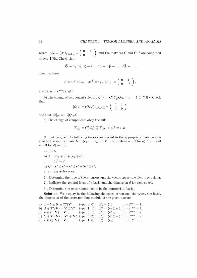
2. Let be given the following tensors, expressed in the appropriate basis, associ-ated to the natural basis B = e1, . . . , en of V = Rn, where n = 2 for a), b), c), andn = 3 for d) and e).
a) a = 5;
b) A = 2e1 ⊗ e2 + 3e2 ⊗ e2;
c) η = 3e2 − e1;
d) Q = e2 ⊗ e3 − e1 ⊗ e2 + 5e2 ⊗ e2;
e) v = 3e1 + 4e2 − e3.
1o. Determine the type of these tensors and the vector space to which they belong.
2o. Indicate the general form of a basis and the dimension d for each space.
3o. Determine the tensor components in the appropriate basis.
Solution. We display in the following the space of tensors, the types, the basis,the dimension of the corresponding module of the given tensors:
a) a = 5 ∈ R ≡ T 00 (V), type (0, 0), B0
0 = 1, d = 20+0 = 1,b) A ∈ T 1
1 (V) = V ⊗V∗, type (1, 1), B11 = ei ⊗ ej, d = 21+1 = 4,
c) η ∈ T 01 (V) = V∗, type (0, 1), B0
1 = ej, d = 20+1 = 2,d) Q ∈ T 0
2 (V) = V∗ ⊗V∗, type (0, 2), B02 = ei ⊗ ej, d = 30+2 = 9,
e) v ∈ T 10 (V) = V, type (1, 0), B1
0 = ei, d = 31+0 = 3,
1.2. TENSORS 13
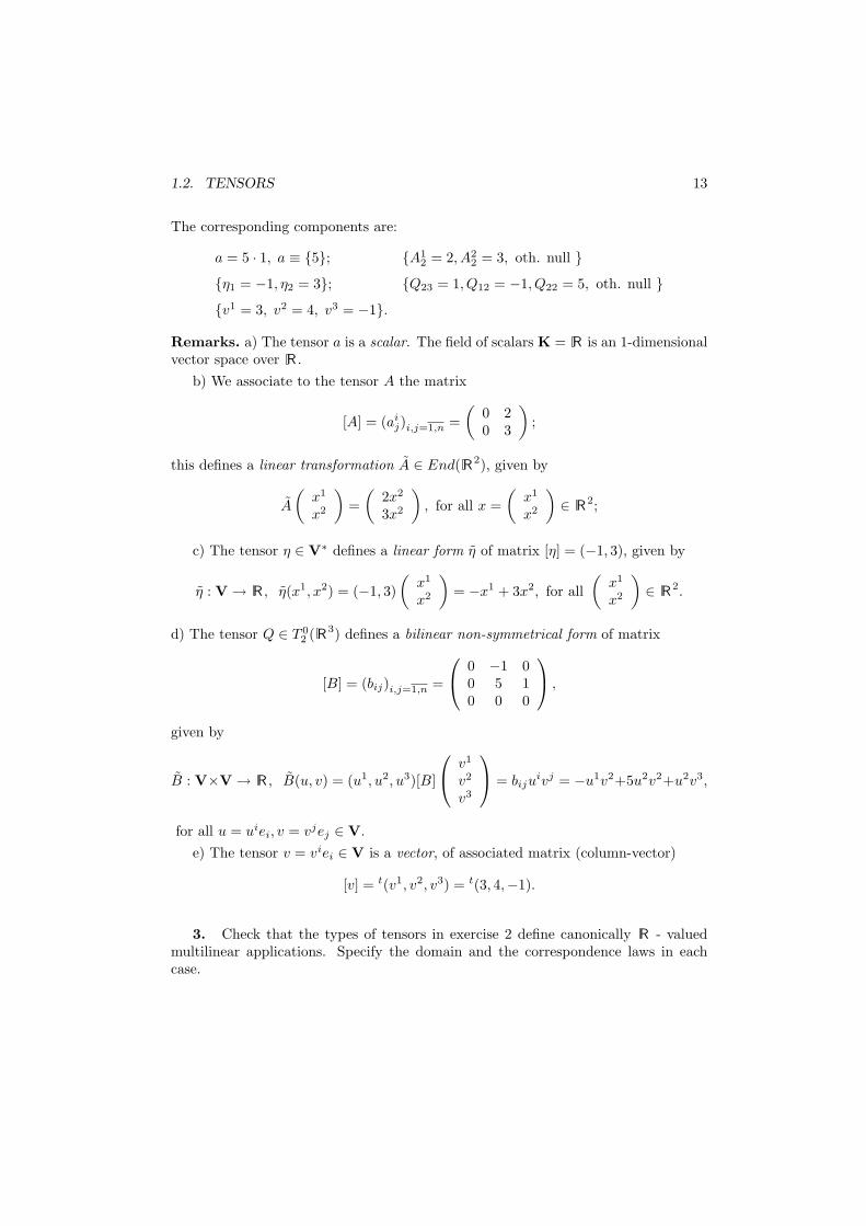
The corresponding components are:
a = 5 · 1, a ≡ 5; A12 = 2, A2
2 = 3, oth. null η1 = −1, η2 = 3; Q23 = 1, Q12 = −1, Q22 = 5, oth. null v1 = 3, v2 = 4, v3 = −1.
Remarks. a) The tensor a is a scalar. The field of scalars K = R is an 1-dimensionalvector space over R .
b) We associate to the tensor A the matrix
[A] = (aij)i,j=1,n =
(0 20 3
);
this defines a linear transformation A ∈ End(R2), given by
A
(x1
x2
)=
(2x2
3x2
), for all x =
(x1
x2
)∈ R2;
c) The tensor η ∈ V∗ defines a linear form η of matrix [η] = (−1, 3), given by
η : V → R , η(x1, x2) = (−1, 3)(
x1
x2
)= −x1 + 3x2, for all
(x1
x2
)∈ R2.
d) The tensor Q ∈ T 02 ( R3) defines a bilinear non-symmetrical form of matrix
[B] = (bij)i,j=1,n =
0 −1 00 5 10 0 0
,
given by
B : V×V → R , B(u, v) = (u1, u2, u3)[B]
v1
v2
v3
= biju
ivj = −u1v2+5u2v2+u2v3,
for all u = uiei, v = vjej ∈ V.e) The tensor v = viei ∈ V is a vector, of associated matrix (column-vector)
[v] = t(v1, v2, v3) = t(3, 4,−1).
3. Check that the types of tensors in exercise 2 define canonically R - valuedmultilinear applications. Specify the domain and the correspondence laws in eachcase.
14 CHAPTER 1. TENSOR ALGEBRA AND ANALYSIS
Solution.
a) a ∈ T 00 (V ) = R ⇒ a : R → R , a(k) = ak ∈ R , ∀k ∈ R .
b) A ∈ T 11 (V ) ⇒ A : V∗ ×V → R , A(η, v) = Ai
jηivj ∈ R ,
∀η ∈ V∗, v ∈ V.c) η ∈ T 0
1 (V ) = V∗ ⇒ η : V → R , η(v) = ηivi ∈ R , ∀v ∈ V.
d) B ∈ T 02 (V ) = V∗ ⊗V∗ ⇒ B : V ⊗V → R , B(v, w) = Bijv
iwj ∈ R ,∀v, w ∈ V,
e) v ∈ T 10 (V ) = V ⇒ v : V∗ → R , v(η) = viηi ∈ R , ∀η ∈ V∗.
4. Compute the following tensors expressed in the corresponding basis associatedto the natural basis B1
0 ⊂ V = Rn:
a) w = 3v + u, where u = e1 − e2, and v ≡ v1 = 5, v2 = 0, v3 = 7, (n = 3);b) R = P + 5Q, where P = e1 ⊗ e3 ⊗ e2 and
Q = e2 ⊗ e1 ⊗ e2 − 5e1 ⊗ e3 ⊗ e2, (n = 3);
c) R = tr21(Q), where
Q = 5e1 ⊗ e2 ⊗ e1 ⊗ e3 − 4e2 ⊗ e2 ⊗ e2 ⊗ e3 − e1 ⊗ e2 ⊗ e2 ⊗ e3, (n = 3);
d) k = tr11(A), where A = 5e1 ⊗ e1 + 6e1 ⊗ e2 − e2 ⊗ e2, (n = 2);
e) w = tr21(T ), where
T = A⊗ v, A = 5e1 ⊗ e2 − 3e2 ⊗ e3, v = 2e2 − e1, (n = 3);
f) k = tr11(η ⊗ v), where
η = e1 + 2e2 and v = 2e2, (n = 2);
g) a = tr11tr
22(B ⊗ u⊗ v), where
B = e1 ⊗ e2 − 2e2 ⊗ e2 and u = e1, v = e2 − 3e1, (n = 2).
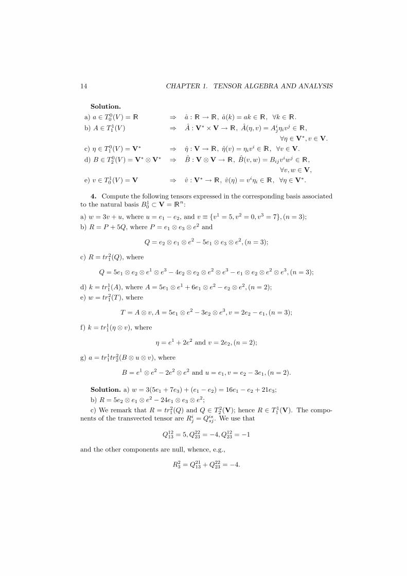
Solution. a) w = 3(5e1 + 7e3) + (e1 − e2) = 16e1 − e2 + 21e3;b) R = 5e2 ⊗ e1 ⊗ e2 − 24e1 ⊗ e3 ⊗ e2;c) We remark that R = tr2
1(Q) and Q ∈ T 22 (V); hence R ∈ T 1
1 (V). The compo-nents of the transvected tensor are Ri
j = Qissj . We use that
Q1213 = 5, Q22
23 = −4, Q1223 = −1
and the other components are null, whence, e.g.,
R23 = Q21
13 + Q2223 = −4.
1.3. RAISING AND LOWERING OF THE INDICES OF A TENSOR 15
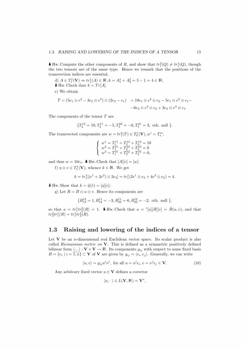
Hw. Compute the other components of R, and show that tr21(Q) 6= tr1
1(Q), thoughthe two tensors are of the same type. Hence we remark that the positions of thetransvection indices are essential.
d) A ∈ T 11 (V) ⇒ tr1
1(A) ∈ R , k = A11 + A2
2 = 5− 1 = 4 ∈ R ;Hw.Check that k = Tr[A].
e) We obtain
T = (5e1 ⊗ e2 − 3e2 ⊗ e3)⊗ (2e2 − e1) = 10e1 ⊗ e2 ⊗ e2 − 5e1 ⊗ e2 ⊗ e1−−6e2 ⊗ e3 ⊗ e2 + 3e2 ⊗ e3 ⊗ e1.
The components of the tensor T are
T 122 = 10, T 11
2 = −5, T 223 = −6, T 21
3 = 3, oth. null .
The transvected components are w = tr21(T ) ∈ T 1
0 (V), wi = T iss ,
w1 = T 111 + T 12
2 + T 133 = 10
w2 = T 211 + T 22
2 + T 233 = 0
w3 = T 311 + T 32
2 + T 333 = 0,
and thus w = 10e1. Hw.Check that [A][v] = [w].f) η ⊗ v ∈ T 1
1 (V), whence k ∈ R . We get
k = tr11[(e
1 + 2e2)⊗ 2e2] = tr11(2e1 ⊗ e2 + 4e2 ⊗ e2) = 4.
Hw. Show that k = η(v) = [η][v];g) Let R = B ⊗ u⊗ v. Hence its components are
R1212 = 1, R11
12 = −3, R1122 = 6, R12
22 = −2, oth. null ,
so that a = tr11tr
22(R) = 1. Hw. Check that a = t[u][B][v] = B(u, v), and that
tr22tr
11(R) = tr1
1tr22(R).
1.3 Raising and lowering of the indices of a tensor
Let V be an n-dimensional real Euclidean vector space. Its scalar product is alsocalled Riemannian metric on V. This is defined as a symmetric positively definedbilinear form 〈·, ·〉 : V×V → R . Its components gij with respect to some fixed basisB = ei | i = 1, n ⊂ V of V are given by gij = 〈ei, ej〉. Generally, we can write
〈u, v〉 = gijuivj , for all u = uiei, v = vjej ∈ V. (10)
Any arbitrary fixed vector u ∈ V defines a covector
〈u, · 〉 ∈ L(V, R) = V∗,
16 CHAPTER 1. TENSOR ALGEBRA AND ANALYSIS
of components gijui, via the linear mapping given by
G : V → V∗, (G(u))(v) = 〈u, v〉, for all u, v ∈ V.
Properties: 1o. The mapping G is linear and bijective, hence an isomorphism.2o. Using (10), one can see that G is characterized by the matrix (denoted also
by G), G = (gij)i,j=1,n, of inverse G−1 = (gkl)k,l=1,n, where gklgls = δks .
3o. If B is an orthonormal basis with respect to the scalar product 〈·, ·〉, we haveG(ei) = ei ∈ V∗, i = 1, n, and we notice that the dual basis B∗ is also orthonormalwith respect to the scalar product on V∗ given by
〈ω, η〉 = ωiηjgij , for all ω = ωie
i, η = ηjej ∈ V∗.
Using G and G−1 one can lower, respectively raise the indices of a given tensor.
1.3.1 Definition. Let T = T i1...ip
j1...jq ∈ T p
q (V ) and s ∈ 1, p and t ∈ 1, q. Thefunction defined by
(Gs,tT )i1...is−1is+1...ip
j1...jt−1jtjt+1...jq+1= gjtisT
i1...is−1isis+1...ip
j1...jt−1jt+1...jq+1
is called lowering of the indices. Analogously, using G−1, we define the raising ofthe indices. The lowering and raising produce new tensors, since they are in fact thetensor products g ⊗ T , g−1 ⊗ T followed by suitable transvections.
The real vector spaces of tensors of order p + q are isomorphic via raising andlowering of indices. For instance one can lower the index of a vector v = viei ∈ V, byvk = gksv
s, obtaining the covector ω = vkek ∈ V∗, or raise the index of a covectorω = ωkek ∈ V∗, by vk = gksωs, obtaining the vector v = vkek ∈ V.
Remark. The scalar product gij on V induces the scalar product gkl on V ∗, andthe scalar product on T p
q (V ) given by the mapping
Gk1l1...kqlqi1j1...ipjp
= gi1j1 . . . gipjp · gk1l1 . . . gkqlq .
1.3.2. Exercises
1. Find a, b, c ∈ R such that the mapping 〈 · , · 〉 : R2 × R2 → R ,
〈u, v〉 = u1v1 − 2au1v2 − 2u2v1 + cu2v2 + b, for all u = (u1, u2), v = (v1, v2) ∈ R2,
defines a scalar product on R2. Find its components relative to the canonic basis.
Solution. The bilinearity implies b = 0, the symmetry implies a = 1 and thepositive definiteness implies c > 4. Hence 〈 · , · 〉 defines a scalar product iff a =1, b = 0, c > 4. In this case we have
〈u, v〉 = u1v1 − 2u1v2 − 2u2v1 + cu2v2, for all u = (u1, u2), v = (v1, v2) ∈ R2,

1.4. VECTOR FIELDS AND COVECTOR FIELDS 17
and its components are (gij)i,j=1,2 =(
1 −2−2 c
).
2. Lower the index of the vector u = 3e1 + 2e2 − e3 ∈ V = R3; raise the indexof the covector ω = 2e1 − 3e3 ∈ V ∗, using the metric
〈u, v〉 = u1v1 + 2u2v2 + 3u3v3, for all u = (u1, u2, u3), v = (v1, v2, v3) ∈ R3.
Solution. The 1-form η = G(u) has the components
η1 = g1sus = g11u
1 = 1 · 3 = 3
η2 = g2sus = g22u
2 = 2 · 2 = 4
η3 = g3sus = g33u
3 = 3 · (−1) = −3,
and consequently η = 3e1 + 4e2 − 3e3. Also, for v = G−1(ω), we obtain
v1 = g1jωj = g11ω1 = 1 · 2 = 2
v2 = g2jωj = g22ω2 = 12 · 0 = 0
v3 = g3jωj = g33ω3 = 13 · (−3) = −1,
and hence v = 2e1 − e3 ∈ V.
3. Lower the third index on first position and raise the second index on positionthree, for a tensor S ∈ T 3
3 (V ), where V is endowed with the metric gij . Raise thesecond index of the metric g on the first position.
Solution. We have
(G31S)irujkl = Sirs
jklgus ∈ T 24 (V ), (G23S)irts
jl = Sirsjklg
kt ∈ T 42 (V ).
We get also (G21g)ij = gisgjs = δi
j .
1.4 Vector fields and covector fields
Classically, a vector field in R3 is given by
~v(x, y, z) = v1(x, y, z)~i + v2(x, y, z)~j + v3(x, y, z)~k.
We shall consider the more general case, the space Rn, and the point x = (x1, . . . , xn) ∈D ⊂ Rn, where D is an open subset of Rn. Also, to avoid repetitions, we assumethe differentiability of class C∞ in definitions.
1.4.1 Definition. A differentiable function f : D → R is called a scalar field.We denote by F(D) the set of all scalar fields on D.
18 CHAPTER 1. TENSOR ALGEBRA AND ANALYSIS
It can be shown that F(D) can be organized as a real commutative algebra 3 ina natural way, considering the addition and multiplication of functions in F(D), andtheir multiplication with real scalars.
1.4.2 Definition. Let x be a fixed point of D ⊂ Rn. If a function Xx : F(D) → Rsatisfies the conditions:
1) Xx is R−linear,2) Xx is a derivation, i.e.,
Xx(fg) = Xx(f) · g(x) + f(x) ·Xx(g), ∀f, g ∈ F(D), (11)
then it is called a tangent vector to D at the point x. The set of all tangent vectorsat x is denoted by TxD.
Example. The mapping ∂∂xi
∣∣x
: F(D) → R , given by(
∂
∂xi
∣∣∣∣x
)(f) =
∂f
∂xi(x), for all f ∈ F(D),
is a tangent vector at x.
Remarks. 1o. For any vector Xx, we have Xx(c) = 0, for any c ∈ F(R), that is,for the constant functions f(x) = c. Indeed, from (11) and f = g = 1, we find
Xx(1 · 1) = 1 ·Xx(1) + 1 ·Xx(1),
whence Xx(1) = 0; then Xx(c) = Xx(c · 1) = cXx(1) = c · 0 = 0, for all c ∈ R .2o. We define the null operator Ox : F(D) → R , by Ox(f) = 0. Then Ox is a
tangent vector at x.3o. If a, b ∈ R and Xx, Yx are tangent vectors, then aXx + bYx is a tangent vector
at x too.4o. By the addition and the multiplication with scalars, the set TxD has a
structure of a real vector space.
1.4.3 Theorem. The set ∂
∂xi
∣∣∣∣x0
, i = 1, n
is a basis for Tx0D. This is called the natural frame at x0.
Proof. First we check the linear independence. Let ai ∈ R , i = 1, n such thatai ∂
∂xi |x0= 0. Applying the tangent vector ai ∂∂xi |x0∈ Tx0D, to the coordinate function
xj , we obtain
0 = Ox0(xj) =
(ai ∂
∂xi
∣∣∣∣x0
)(xj
)= ai ∂xj
∂xi(x0) = aiδj
i = aj .
3An algebra is a vector space which is endowed with a third (internal multiplicative) operationwhich is associative, distributive with respect to the addition of vectors, and associative with respectto multiplication with scalars.
1.4. VECTOR FIELDS AND COVECTOR FIELDS 19
Thus we have aj = 0, j = 1, n, whence the set is linearly independent.
Now we check that the set
∂∂xi
∣∣x0
, i = 1, n
generates (spans) the space Tx0D.Let f ∈ F(D). Then, applying the rule of derivation of composed functions, we have
f(x) = f(x0) +∫ 1
0
ddt
f (x0 + t(x− x0)) dt =
= f(x0) +∫ 1
0
n∑
i=1
∂f
∂xi
∣∣∣∣x0+t(x−x0)
(xi − xi0)dt.
Denoting gi(x) =∫ 1
0
∂f
∂xi|x0+t(x−x0) dt, we notice that
gi(x0) =∂f
∂xi(x0),
and f(x) = f(x0) +n∑
i=1
gi(x)(xi − xi0). Then applying an arbitrary tangent vector
Xx ∈ TxD to this function, we obtain
Xx(f) = 0 +n∑
i=1
[Xx(gi)(x)(xi − xi
0) + gi(x)Xx(xi − xi0)
],
which becomes, for x = x0,
Xx0(f) =n∑
i=1
Xx0(xi)
∂f
∂xi(x0).
Denoting ai = Xx0(xi) we have
Xx0(f) = ai ∂
∂xi
∣∣∣∣x0
(f).
Since f is arbitrary, we infer Xx0 = ai ∂
∂xi|x0 , whence Xx0 is generated by the set
∂
∂xi
∣∣x0
, i = 1, n
. 2
Example. The object XP = 2 ∂∂x |P +3 ∂
∂y |P∈ TP D, is a tangent vector at thepoint P (x0, y0) ∈ D ⊂ R2, which is decomposed with respect to the basis
∂
∂x
∣∣∣∣P
,∂
∂y
∣∣∣∣P
⊂ TP D.
1.4.4 Definition. Let D ⊂ Rn. A differentiable function X : D → ⋃x∈D
TxD,
with X(x) ∈ TxD, for each x ∈ D, is called a vector field on D. We denote by X (D)the set of all vector fields on D.
20 CHAPTER 1. TENSOR ALGEBRA AND ANALYSIS
The operations
(X + Y )(x) = X(x) + Y (x)(λX)(x) = λX(x), for all λ ∈ R , X, Y ∈ X (D), x ∈ D,
determine on X (D) a structure of a real vector space.A basis of the F(D)−module 4 X (D) is provided by the set of vector fields
∂∂xi , i = 1, n, where
∂
∂xi: D →
⋃
x∈D
TxD,∂
∂xi(x) =
∂
∂xi
∣∣∣∣x
, for all x ∈ D, i = 1, n. (12)
They determine a natural field of frames for X (D), and are called fundamental vectorfields.
1.4.5 Theorem. Let X ∈ X (D). There exist the real functions
Xi ∈ F(D), i = 1, n,
such that X = Xi ∂∂xi .
The differentiable functions Xi are called the components of the vector field Xwith respect to the natural frame field.
Proof. For x ∈ D, X(x) = Xi(x) ∂∂xi |x, Xi(x) ∈ R , i = 1, n. Thus
Xi : x ∈ D → Xi(x) ∈ R , i = 1, n
are the required components. 2
Example. X = xx2+y2
∂∂x + exy ∂
∂y ∈ X (D), where D = R2\(0, 0) ⊂ R2, is avector field on D.
1.4.6 Definition. Let X, Y ∈ X (D) be two vector fields (having their componentsXi, Y j of class C∞). We call the Lie bracket of X and Y , the field [X,Y ] ∈ X (D)given by
[X,Y ](f) = X(Y (f))− Y (X(f)), for all f ∈ F(D), (13)
where we denoted X(f) = Xi ∂f∂xi , for all f ∈ F(D).
The following properties hold true:a) [X,Y ] = −[Y, X],b) [X, [Y, Z]] + [Y, [Z,X]] + [Z, [X, Y ]] = 0, (the Jacobi identity);c) [X, X] = 0, for all X, Y, Z ∈ X (D),
and we have a) ⇔ c). Also, the Lie bracket is R -bilinear with respect to X and Y .
4We call an R−module a set M endowed with two operations (one internal - addition, and thesecond external - multiplication with scalars from R), which obey the same properties as the ones ofa vector space, with the essential difference that R is not a field, but a ring.
1.4. VECTOR FIELDS AND COVECTOR FIELDS 21
The real vector space X (D) together with the product given by the bracket
[ . , . ] : X (D)×X (D) → X (D)
defined in (13) determine a real Lie algebra.For D ⊂ R3, any vector field v ∈ X (D) can be rewritten in the classical sense
v(x, y, z) = v1(x, y, z)~i + v2(x, y, z)~j + v3(x, y, z)~k,
with v1, v2, v3 ∈ F(D), replacing
∂
∂x,
∂
∂y,
∂
∂z
with ~i,~j,~k.
For any x0 ∈ D ⊂ Rn, consider the dual vector space (Tx0D)∗ and denote itby T ∗x0
D. Its elements are the linear mappings ωx0 ∈ T ∗x0D, ωx0 : Tx0D → R
called covectors (covariant vectors, 1−forms) at x0. The space T ∗x0D has a canonical
structure of a vector space and is called the cotangent space.
Example. For a given mapping f ∈ F(D), for each x0 ∈ D, its differentialdf |x0∈ T ∗x0
D at x0 is an R - linear mapping on Tx0D, hence an example of covectorat x0, since
(df |x0)(Xx0) = Xx0(f), for all Xx0 ∈ Tx0D.
Theorem. Let
∂
∂xi
∣∣∣∣x0
, i = 1, n
be the natural frame in Tx0D, and xj : D →
R the coordinate functions. Then the set
dxi |x0 , i = 1, nis a basis in T ∗x0
D, called also (natural) coframe at x0.
Proof. We remark that dxj |x0
(∂
∂xi|x0
)=
∂xj
∂xi(x0) = δj
i , i.e., we have a dual
basis. Now we want to analyse directly if the given set is a basis. Consider thevanishing linear combination ajdxj |x0= 0, aj ∈ R , j = 1, n. Applying this covector
to∂
∂xi
∣∣∣∣x0
, we obtain
0 = (ajdxj |x0)
(∂
∂xi
∣∣∣∣x0
)= ajδ
ji = ai ⇔ ai = 0, i = 1, n,
hence the set of covectors is linearly independent.Consider now a covector ωx0 ∈ T ∗x0
D. Since ωx0 : Tx0D → R is linear, for any
tangent vector Xx0 = Xix0
∂
∂xi|x0∈ Tx0D, we have
ωx0(Xx0) = ωx0
(Xi
x0
∂
∂xi
∣∣∣∣x
)= Xi
x0ωx0
(∂
∂xi
∣∣∣∣x0
).
22 CHAPTER 1. TENSOR ALGEBRA AND ANALYSIS
Similarly, for any i = 1, n, we find
dxi |x0 (Xxo) = dxi |x0
(Xk
x0
∂
∂xk
∣∣∣∣x0
)= Xk
x0dxi |x0
(∂
∂xk
∣∣∣∣x0
)= Xk
x0δik = Xi
x0,
whence, denoting ωi(x0) = ωx0
(∂
∂xi
∣∣x0
), we infer
ωx0(Xx0) = ωi(x0)dxi |x0 (Xx0) = (ωi(x0)dxi |x0)(Xx0), for all Xx0 ∈ Tx0D.
Thus, the covector decomposes ωx0 = ωi(x0)dxi |x0 , and hence is generated by theset dxi |x0 , i = 1, n. 2
Definition. A differentiable mapping ω : D → ∪x∈D
T ∗x D, with ω(x) ∈ T ∗x D is
called differential 1-form (or covariant vector field, covector field on D). The set ofdifferential 1-forms on D will be denoted by X ∗(D).
The addition of forms and their multiplication with real scalar functions endowsX ∗(D) with a structure of a real vector space. The set of 1-forms
dxi : D →⋃
x∈D
T ∗x D, dxi(x) = dxi |x, for all x ∈ D, i = 1, n (14)
determines a basis in the F(D)-module X ∗(D). Any differential 1−form can bewritten ω = ωidxi. The components ωi are differentiable functions.
Examples. 1. ωx = 2dx1 |x +3dx2 |x∈ T ∗x D, x ∈ D ⊂ Rn is a covector.
2. Xx = 5 ∂∂x1 |x − ∂
∂x2 |x∈ TxD is a vector.3. ω = x1x2dx1 − (sinx2)dx2 ∈ X ∗(D) is a covector field (1-form).4. X = e−x2 ∂
∂x1 + x2∂
∂x3 ∈ X (D), where D ⊂ R3, is a vector field.
1.4.7 Let (x1, . . . , xn) be the coordinates of an arbitrary point x ∈ D ⊂ Rn. Ifthe point x has the new coordinates (x1′ , . . . , xn′), then these are related to the oldones by a change of coordinates
xi′ = xi′(xi), i′ = 1, n, det
(∂xi′
∂xi(xj)
)6= 0 (15)
which are reverted locally to
xi = xi(xi′), i = 1, n, det(
∂xi
∂xi′ (xj′)
)6= 0. (16)
Then the transformation (16) induces a change of basis in TxD,
Bx =
∂
∂xi
∣∣∣∣x
, i = 1, n
→ B′
x =
∂
∂xi′
∣∣∣∣x
, i′ = 1, n
,
1.4. VECTOR FIELDS AND COVECTOR FIELDS 23
and also of the corresponding dual basis in T ∗x D,
B∗x = dxi |x, i = 1, n → B∗′
x dxi′ |x, i = 1, n.
Proposition. The bases above are pairwise related by the formulas
∂
∂xi
∣∣∣∣x
=∂xi′
∂xi(xj)
∂
∂xi′
∣∣∣∣x
, i = 1, n
dxi |x =∂xi
∂xi′ (xj′)dxi′ |x , i = 1, n.
The corresponding bases of fields of frames of the F(D)-modules X (D) and X ∗(D),are respectively
B =
∂
∂xi, i = 1, n
, B′ =
∂
∂xi′ , i′ = 1, n
,
andB∗ = dxi, i = 1, n, B∗′ = dxi′ , i = 1, n.
They are related by
∂
∂xi=
∂xi′
∂xi(xj)
∂
∂xi′ ; dxi =∂xi
∂xi′ (xj′)dxi′ . (17)
Let X ∈ X (D), X = Xi ∂∂xi = Xi′ ∂
∂xi′ be a vector field, and let
ω ∈ X ∗(D), ω = ωidxi = ωi′dxi′
be an 1-form on D.Then their old/new components of X and ω are respectively related by
Xi′ =∂xi′
∂xiXi, ωi′ =
∂xi
∂xi′ ωi.
Remark. Consider a point P = (x, y) ∈ D ⊂ R2, and a vector field
X = f∂
∂x+ g
∂
∂y∈ X (D), f, g ∈ F(D).
We may identify ∂∂x , ∂
∂y ≡ ~i,~j, since the vectors ∂∂x |P and ∂
∂x |Q are equipolent
for all P, Q ∈ D; ~i is exactly the class of equipolence ∂∂x ; the similar happens to ∂
∂y .
Therefore we can write X = f~i + g~j.When the metric on D ⊂ R2 is the canonic metric, gij = δij , i, j = 1, 2, we might
also identify dx, dy ≡ ~i,~j, respectively.
24 CHAPTER 1. TENSOR ALGEBRA AND ANALYSIS
Similar considerations hold true for D ⊂ R3, where we identify ∂∂x , ∂
∂y , ∂∂z ≡
~i,~j,~k, and, in the case of canonic metric, dx, dy, dz ≡ ~i,~j,~k.Example. We consider in D = R2\(0, 0) the change of coordinates
(x1, x2) ≡ (x, y) ∈ R2\(0, 0) → (x1′ , x2′) ≡ (ρ, θ) ∈ (0,∞)× [0, 2π),
given by xi = xi(xi′), i = 1, 2, with
x1 = x1′ cos x2′
x2 = x1′ sin x2′ or
x = ρ cos θy = ρ sin θ.
Then the change of basis B = ∂∂x , ∂
∂y → B′ = ∂∂ρ , ∂
∂θ is described by the relations
∂
∂x=
∂ρ
∂x
∂
∂ρ+
∂θ
∂x
∂
∂θ,
∂
∂y=
∂ρ
∂y
∂
∂ρ+
∂θ
∂y
∂
∂θ.
and the change of dual bases B∗ → B∗′ is performed according to the rules
dx =∂x
∂ρdρ +
∂x
∂θdθ, dy =
∂y
∂ρdρ +
∂y
∂θdθ.
1.4.8. Exercises
1. Let be the vector field
X = x∂
∂x+ y
∂
∂y+ z
∂
∂z∈ X (D), D ⊂ R3.
Find the components of X in cylindrical and spherical coordinates.
Solution. Let be the change from Cartesian to cylindrical coordinates
(x1, x2, x3) ≡ (x, y, z) → (x1′ , x2′ , x3′) = (ρ, θ, z),
given by the formulas
x = ρ cos θy = ρ sin θz = z
⇔
x1 = x1′ cosx2′
x2 = x1′ sin x2′
x3 = x3′⇒
ρ =√
x2 + y2
θ = arctan yx
z = z.(18)
Since the vector field rewrites
X = x1 ∂
∂x1+ x2 ∂
∂x2+ x3 ∂
∂x3,
we get the components X1 = x1, X2 = x2, X3 = x3. We have to determine thenew components X1′ , X2′ , X3′ , which satisfy X = Xi′ ∂
∂xi′ , by means of the relationswhich link the two sets of components of X:
Xi =∂xi
∂xi′ Xi′ , Xi′ =
∂xi′
∂xiXi, i, i′ = 1, 3. (19)
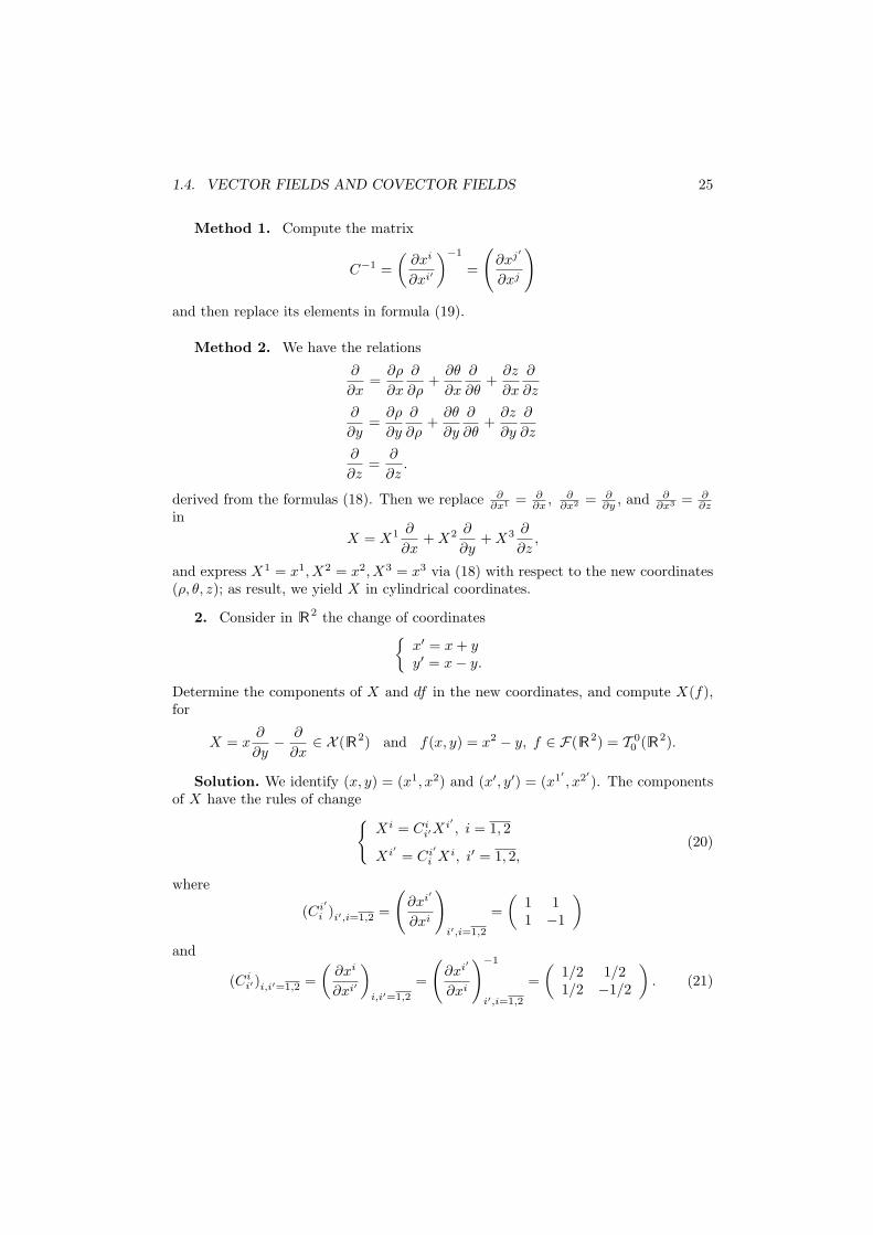
1.4. VECTOR FIELDS AND COVECTOR FIELDS 25
Method 1. Compute the matrix
C−1 =(
∂xi
∂xi′
)−1
=
(∂xj′
∂xj
)
and then replace its elements in formula (19).
Method 2. We have the relations
∂
∂x=
∂ρ
∂x
∂
∂ρ+
∂θ
∂x
∂
∂θ+
∂z
∂x
∂
∂z
∂
∂y=
∂ρ
∂y
∂
∂ρ+
∂θ
∂y
∂
∂θ+
∂z
∂y
∂
∂z
∂
∂z=
∂
∂z.
derived from the formulas (18). Then we replace ∂∂x1 = ∂
∂x , ∂∂x2 = ∂
∂y , and ∂∂x3 = ∂
∂zin
X = X1 ∂
∂x+ X2 ∂
∂y+ X3 ∂
∂z,
and express X1 = x1, X2 = x2, X3 = x3 via (18) with respect to the new coordinates(ρ, θ, z); as result, we yield X in cylindrical coordinates.
2. Consider in R2 the change of coordinates
x′ = x + yy′ = x− y.
Determine the components of X and df in the new coordinates, and compute X(f),for
X = x∂
∂y− ∂
∂x∈ X ( R2) and f(x, y) = x2 − y, f ∈ F(R2) = T 0
0 (R2).
Solution. We identify (x, y) = (x1, x2) and (x′, y′) = (x1′ , x2′). The componentsof X have the rules of change
Xi = Ci
i′Xi′ , i = 1, 2
Xi′ = Ci′i Xi, i′ = 1, 2,
(20)
where
(Ci′i )i′,i=1,2 =
(∂xi′
∂xi
)
i′,i=1,2
=(
1 11 −1
)
and
(Cii′)i,i′=1,2 =
(∂xi
∂xi′
)
i,i′=1,2
=
(∂xi′
∂xi
)−1
i′,i=1,2
=(
1/2 1/21/2 −1/2
). (21)
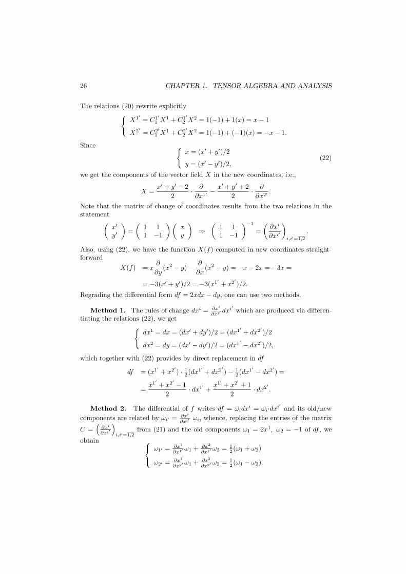
26 CHAPTER 1. TENSOR ALGEBRA AND ANALYSIS
The relations (20) rewrite explicitly
X1′ = C1′1 X1 + C1′
2 X2 = 1(−1) + 1(x) = x− 1
X2′ = C2′1 X1 + C2′
2 X2 = 1(−1) + (−1)(x) = −x− 1.
Since x = (x′ + y′)/2
y = (x′ − y′)/2,(22)
we get the components of the vector field X in the new coordinates, i.e.,
X =x′ + y′ − 2
2· ∂
∂x1′ −x′ + y′ + 2
2· ∂
∂x2′ .
Note that the matrix of change of coordinates results from the two relations in thestatement
(x′
y′
)=
(1 11 −1
) (xy
)⇒
(1 11 −1
)−1
=(
∂xi
∂xi′
)
i,i′=1,2
.
Also, using (22), we have the function X(f) computed in new coordinates straight-forward
X(f) = x∂
∂y(x2 − y)− ∂
∂x(x2 − y) = −x− 2x = −3x =
= −3(x′ + y′)/2 = −3(x1′ + x2′)/2.
Regrading the differential form df = 2xdx− dy, one can use two methods.
Method 1. The rules of change dxi = ∂xi
∂xi′ dxi′ which are produced via differen-tiating the relations (22), we get
dx1 = dx = (dx′ + dy′)/2 = (dx1′ + dx2′)/2
dx2 = dy = (dx′ − dy′)/2 = (dx1′ − dx2′)/2,
which together with (22) provides by direct replacement in df
df = (x1′ + x2′) · 12 (dx1′ + dx2′)− 1
2 (dx1′ − dx2′) =
=x1′ + x2′ − 1
2· dx1′ +
x1′ + x2′ + 12
· dx2′ .
Method 2. The differential of f writes df = ωidxi = ωi′dxi′ and its old/newcomponents are related by ωi′ = ∂xi
∂xi′ ωi, whence, replacing the entries of the matrix
C =(
∂xi
∂xi′
)i,i′=1,2
from (21) and the old components ω1 = 2x1, ω2 = −1 of df , we
obtain
ω1′ = ∂x1
∂x1′ ω1 + ∂x2
∂x1′ ω2 = 12 (ω1 + ω2)
ω2′ = ∂x1
∂x2′ ω1 + ∂x2
∂x2′ ω2 = 12 (ω1 − ω2).
1.4. VECTOR FIELDS AND COVECTOR FIELDS 27
Hence we find
df = ω1′dx1′ + ω2′dx2′ =
=x1′ + x2′ − 1
2· dx1′ +
x1′ + x2′ + 12
· dx2′ .
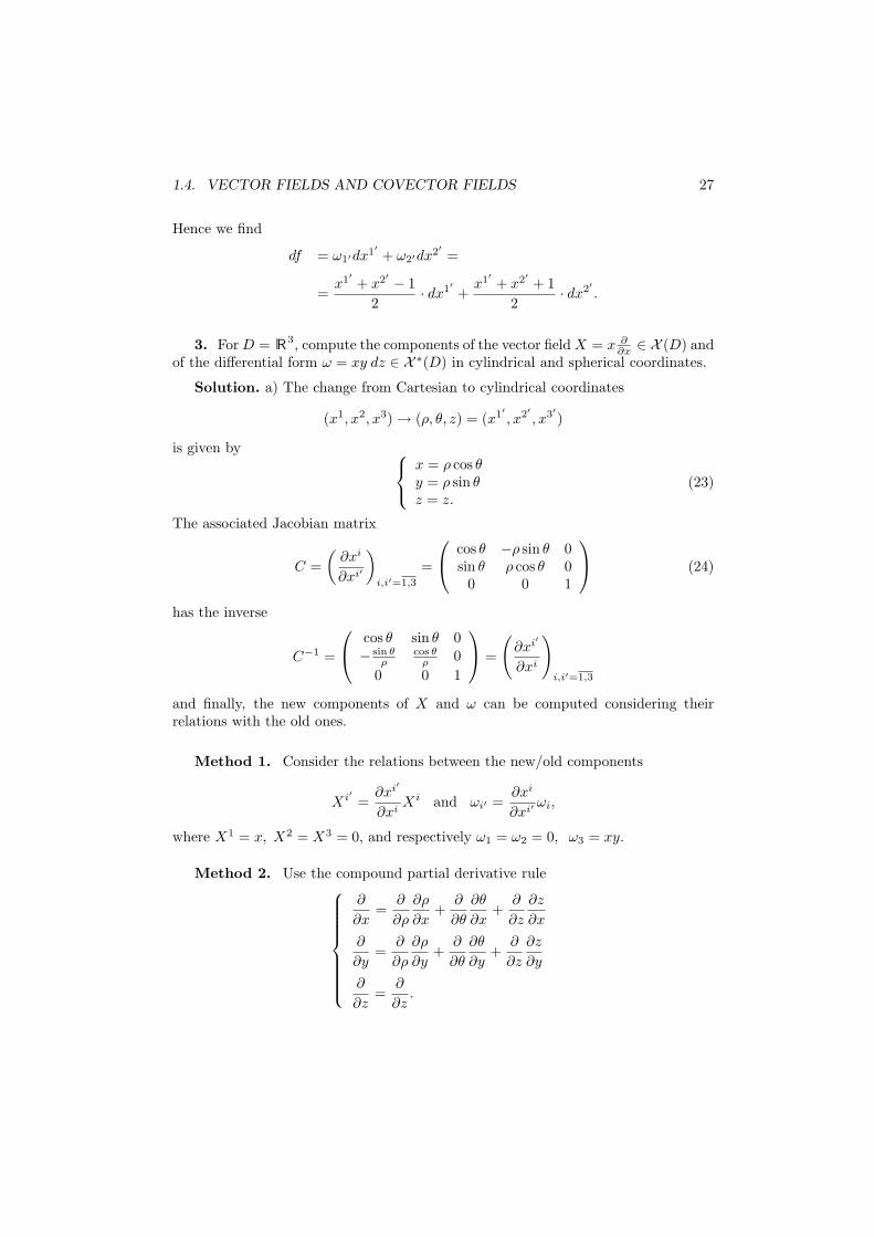
3. For D = R3, compute the components of the vector field X = x ∂∂x ∈ X (D) and
of the differential form ω = xy dz ∈ X ∗(D) in cylindrical and spherical coordinates.
Solution. a) The change from Cartesian to cylindrical coordinates
(x1, x2, x3) → (ρ, θ, z) = (x1′ , x2′ , x3′)
is given by
x = ρ cos θy = ρ sin θz = z.
(23)
The associated Jacobian matrix
C =(
∂xi
∂xi′
)
i,i′=1,3
=
cos θ −ρ sin θ 0sin θ ρ cos θ 0
0 0 1
(24)
has the inverse
C−1 =
cos θ sin θ 0− sin θ
ρcos θ
ρ 00 0 1
=
(∂xi′
∂xi
)
i,i′=1,3
and finally, the new components of X and ω can be computed considering theirrelations with the old ones.
Method 1. Consider the relations between the new/old components
Xi′ =∂xi′
∂xiXi and ωi′ =
∂xi
∂xi′ ωi,
where X1 = x, X2 = X3 = 0, and respectively ω1 = ω2 = 0, ω3 = xy.
Method 2. Use the compound partial derivative rule
∂
∂x=
∂
∂ρ
∂ρ
∂x+
∂
∂θ
∂θ
∂x+
∂
∂z
∂z
∂x
∂
∂y=
∂
∂ρ
∂ρ
∂y+
∂
∂θ
∂θ
∂y+
∂
∂z
∂z
∂y
∂
∂z=
∂
∂z.
28 CHAPTER 1. TENSOR ALGEBRA AND ANALYSIS
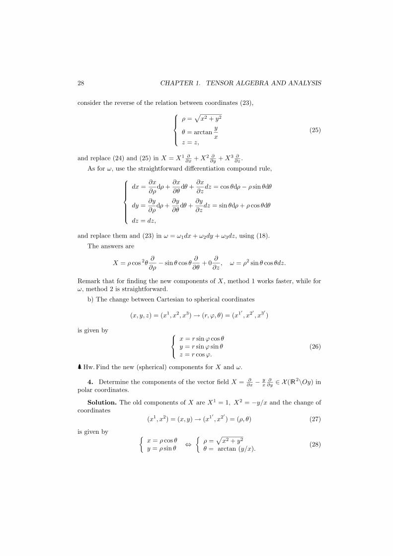
consider the reverse of the relation between coordinates (23),
ρ =√
x2 + y2
θ = arctany
xz = z,
(25)
and replace (24) and (25) in X = X1 ∂∂x + X2 ∂
∂y + X3 ∂∂z .
As for ω, use the straightforward differentiation compound rule,
dx =∂x
∂ρdρ +
∂x
∂θdθ +
∂x
∂zdz = cos θdρ− ρ sin θdθ
dy =∂y
∂ρdρ +
∂y
∂θdθ +
∂y
∂zdz = sin θdρ + ρ cos θdθ
dz = dz,
and replace them and (23) in ω = ω1dx + ω2dy + ω3dz, using (18).
The answers are
X = ρ cos 2θ∂
∂ρ− sin θ cos θ
∂
∂θ+ 0
∂
∂z, ω = ρ2 sin θ cos θdz.
Remark that for finding the new components of X, method 1 works faster, while forω, method 2 is straightforward.
b) The change between Cartesian to spherical coordinates
(x, y, z) = (x1, x2, x3) → (r, ϕ, θ) = (x1′ , x2′ , x3′)
is given by
x = r sin ϕ cos θy = r sinϕ sin θz = r cos ϕ.
(26)
Hw. Find the new (spherical) components for X and ω.
4. Determine the components of the vector field X = ∂∂x − y
x∂∂y ∈ X ( R2\Oy) in
polar coordinates.
Solution. The old components of X are X1 = 1, X2 = −y/x and the change ofcoordinates
(x1, x2) = (x, y) → (x1′ , x2′) = (ρ, θ) (27)
is given by x = ρ cos θy = ρ sin θ
⇔
ρ =√
x2 + y2
θ = arctan (y/x).(28)
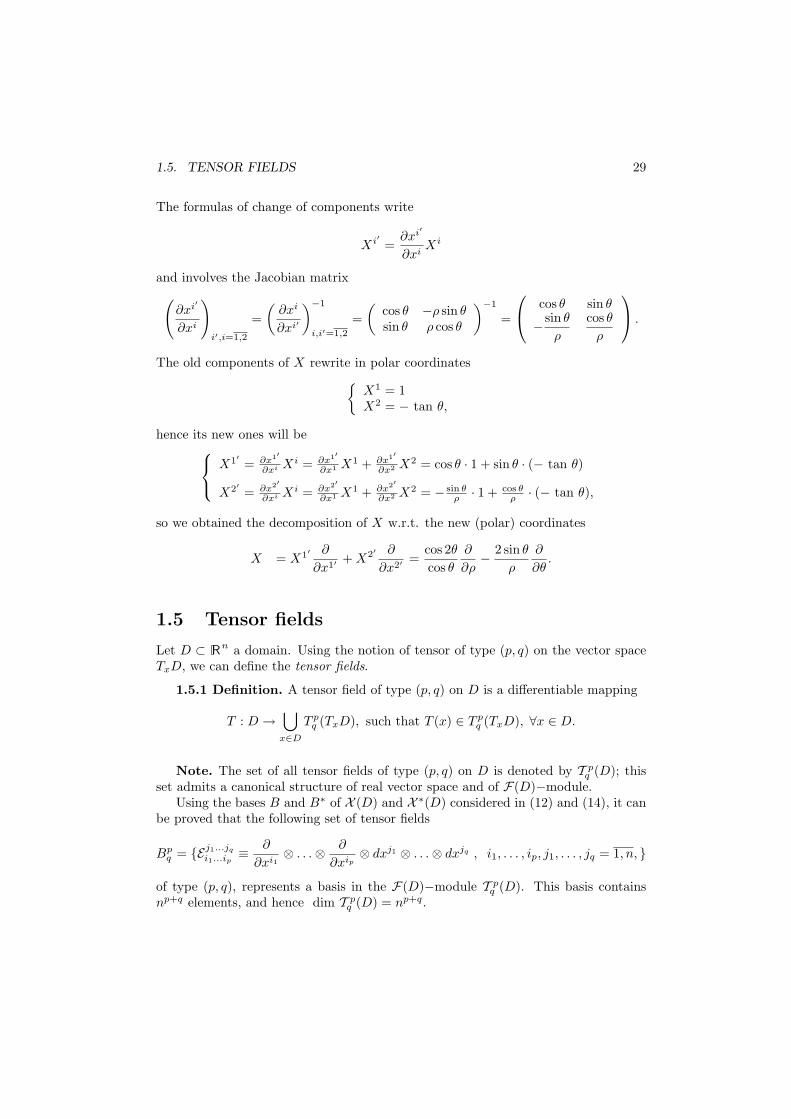
1.5. TENSOR FIELDS 29
The formulas of change of components write
Xi′ =∂xi′
∂xiXi
and involves the Jacobian matrix(
∂xi′
∂xi
)
i′,i=1,2
=(
∂xi
∂xi′
)−1
i,i′=1,2
=(
cos θ −ρ sin θsin θ ρ cos θ
)−1
=
cos θ sin θ
− sin θ
ρ
cos θ
ρ
.
The old components of X rewrite in polar coordinates
X1 = 1X2 = − tan θ,
hence its new ones will be
X1′ = ∂x1′
∂xi Xi = ∂x1′
∂x1 X1 + ∂x1′
∂x2 X2 = cos θ · 1 + sin θ · (− tan θ)
X2′ = ∂x2′
∂xi Xi = ∂x2′
∂x1 X1 + ∂x2′
∂x2 X2 = − sin θρ · 1 + cos θ
ρ · (− tan θ),
so we obtained the decomposition of X w.r.t. the new (polar) coordinates
X = X1′ ∂
∂x1′ + X2′ ∂
∂x2′ =cos 2θ
cos θ
∂
∂ρ− 2 sin θ
ρ
∂
∂θ.
1.5 Tensor fields
Let D ⊂ Rn a domain. Using the notion of tensor of type (p, q) on the vector spaceTxD, we can define the tensor fields.
1.5.1 Definition. A tensor field of type (p, q) on D is a differentiable mapping
T : D →⋃
x∈D
T pq (TxD), such that T (x) ∈ T p
q (TxD), ∀x ∈ D.
Note. The set of all tensor fields of type (p, q) on D is denoted by T pq (D); this
set admits a canonical structure of real vector space and of F(D)−module.Using the bases B and B∗ of X (D) and X ∗(D) considered in (12) and (14), it can
be proved that the following set of tensor fields
Bpq = Ej1...jq
i1...ip≡ ∂
∂xi1⊗ . . .⊗ ∂
∂xip⊗ dxj1 ⊗ . . .⊗ dxjq , i1, . . . , ip, j1, . . . , jq = 1, n,
of type (p, q), represents a basis in the F(D)−module T pq (D). This basis contains
np+q elements, and hence dim T pq (D) = np+q.
30 CHAPTER 1. TENSOR ALGEBRA AND ANALYSIS
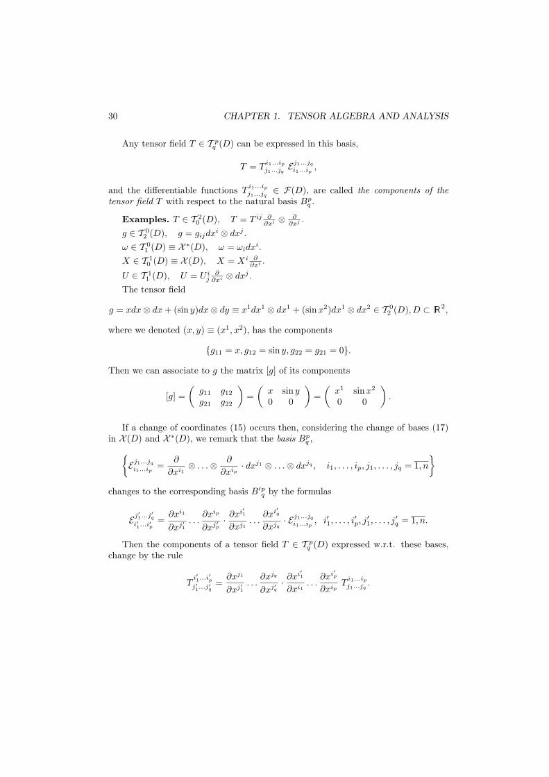
Any tensor field T ∈ T pq (D) can be expressed in this basis,
T = Ti1...ip
j1...jqEj1...jq
i1...ip,
and the differentiable functions Ti1...ip
j1...jq∈ F(D), are called the components of the
tensor field T with respect to the natural basis Bpq .
Examples. T ∈ T 20 (D), T = T ij ∂
∂xi ⊗ ∂∂xj .
g ∈ T 02 (D), g = gijdxi ⊗ dxj .
ω ∈ T 01 (D) ≡ X ∗(D), ω = ωidxi.
X ∈ T 10 (D) ≡ X (D), X = Xi ∂
∂xi .
U ∈ T 11 (D), U = U i
j∂
∂xi ⊗ dxj .The tensor field
g = xdx⊗ dx + (sin y)dx⊗ dy ≡ x1dx1 ⊗ dx1 + (sin x2)dx1 ⊗ dx2 ∈ T 02 (D), D ⊂ R2,
where we denoted (x, y) ≡ (x1, x2), has the components
g11 = x, g12 = sin y, g22 = g21 = 0.
Then we can associate to g the matrix [g] of its components
[g] =(
g11 g12
g21 g22
)=
(x sin y0 0
)=
(x1 sin x2
0 0
).
If a change of coordinates (15) occurs then, considering the change of bases (17)in X (D) and X ∗(D), we remark that the basis Bp
q ,
Ej1...jq
i1...ip=
∂
∂xi1⊗ . . .⊗ ∂
∂xip· dxj1 ⊗ . . .⊗ dxjq , i1, . . . , ip, j1, . . . , jq = 1, n
changes to the corresponding basis B′pq by the formulas
Ej′1...j′qi′1...i′p
=∂xi1
∂xj′1. . .
∂xip
∂xj′p· ∂xi′1
∂xj1. . .
∂xi′q
∂xjq· Ej1...jq
i1...ip, i′1, . . . , i
′p, j
′1, . . . , j
′q = 1, n.
Then the components of a tensor field T ∈ T pq (D) expressed w.r.t. these bases,
change by the rule
Ti′1...i′pj′1...j′q
=∂xj1
∂xj′1. . .
∂xjq
∂xj′q· ∂xi′1
∂xi1. . .
∂xi′p
∂xipT
i1...ip
j1...jq.
1.5. TENSOR FIELDS 31
1.5.2. Exercises
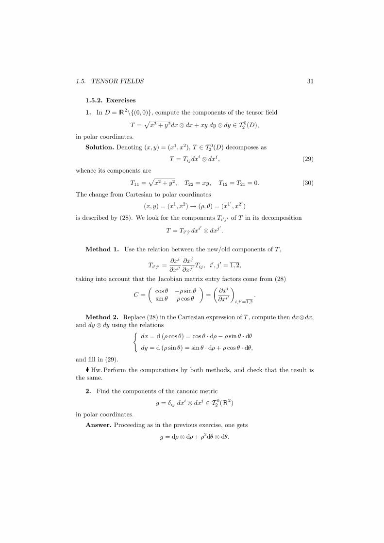
1. In D = R2\(0, 0), compute the components of the tensor field
T =√
x2 + y2dx⊗ dx + xy dy ⊗ dy ∈ T 02 (D),
in polar coordinates.
Solution. Denoting (x, y) = (x1, x2), T ∈ T 02 (D) decomposes as
T = Tijdxi ⊗ dxj , (29)
whence its components are
T11 =√
x2 + y2, T22 = xy, T12 = T21 = 0. (30)
The change from Cartesian to polar coordinates
(x, y) = (x1, x2) → (ρ, θ) = (x1′ , x2′)
is described by (28). We look for the components Ti′j′ of T in its decomposition
T = Ti′j′dxi′ ⊗ dxj′ .
Method 1. Use the relation between the new/old components of T ,
Ti′j′ =∂xi
∂xi′∂xj
∂xj′ Tij , i′, j′ = 1, 2,
taking into account that the Jacobian matrix entry factors come from (28)
C =(
cos θ −ρ sin θsin θ ρ cos θ
)=
(∂xi
∂xi′
)
i,i′=1,2
.
Method 2. Replace (28) in the Cartesian expression of T , compute then dx⊗dx,and dy ⊗ dy using the relations
dx = d (ρ cos θ) = cos θ · dρ− ρ sin θ · dθ
dy = d (ρ sin θ) = sin θ · dρ + ρ cos θ · dθ,
and fill in (29).
Hw.Perform the computations by both methods, and check that the result isthe same.
2. Find the components of the canonic metric
g = δij dxi ⊗ dxj ∈ T 02 (R2)
in polar coordinates.
Answer. Proceeding as in the previous exercise, one gets
g = dρ⊗ dρ + ρ2dθ ⊗ dθ.
32 CHAPTER 1. TENSOR ALGEBRA AND ANALYSIS
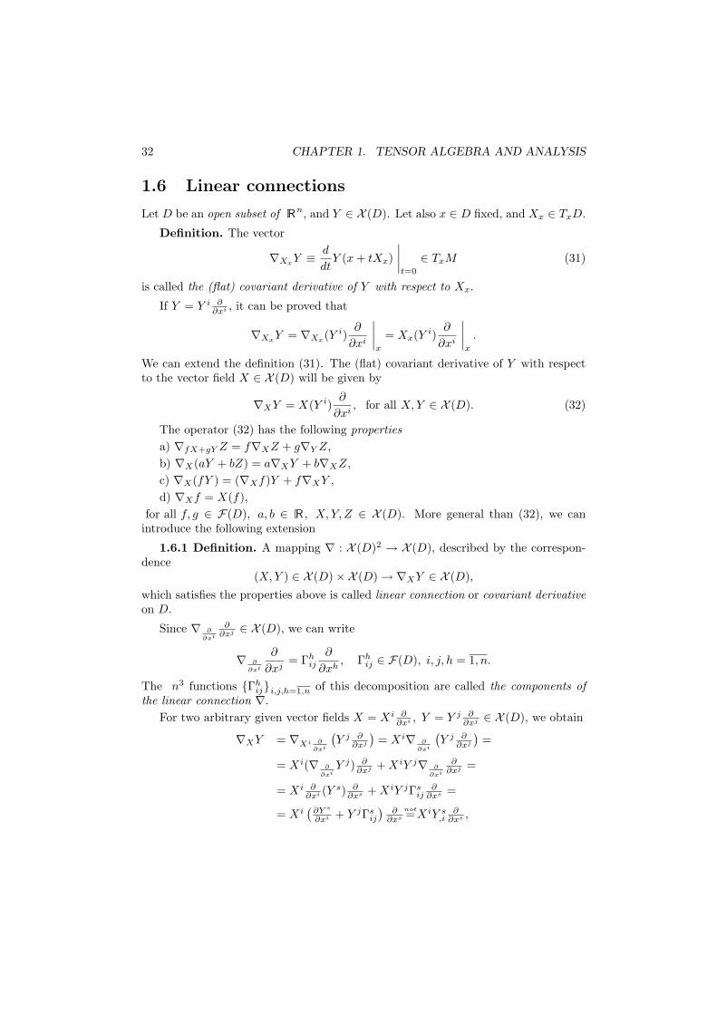
1.6 Linear connections
Let D be an open subset of Rn, and Y ∈ X (D). Let also x ∈ D fixed, and Xx ∈ TxD.
Definition. The vector
∇XxY ≡ d
dtY (x + tXx)
∣∣∣∣t=0
∈ TxM (31)
is called the (flat) covariant derivative of Y with respect to Xx.
If Y = Y i ∂∂xi , it can be proved that
∇XxY = ∇Xx(Y i)∂
∂xi
∣∣∣∣x
= Xx(Y i)∂
∂xi
∣∣∣∣x
.
We can extend the definition (31). The (flat) covariant derivative of Y with respectto the vector field X ∈ X (D) will be given by
∇XY = X(Y i)∂
∂xi, for all X, Y ∈ X (D). (32)
The operator (32) has the following propertiesa) ∇fX+gY Z = f∇XZ + g∇Y Z,b) ∇X(aY + bZ) = a∇XY + b∇XZ,c) ∇X(fY ) = (∇Xf)Y + f∇XY ,d) ∇Xf = X(f),
for all f, g ∈ F(D), a, b ∈ R , X, Y, Z ∈ X (D). More general than (32), we canintroduce the following extension
1.6.1 Definition. A mapping ∇ : X (D)2 → X (D), described by the correspon-dence
(X,Y ) ∈ X (D)×X (D) → ∇XY ∈ X (D),which satisfies the properties above is called linear connection or covariant derivativeon D.
Since ∇ ∂
∂xi
∂∂xj ∈ X (D), we can write
∇ ∂
∂xi
∂
∂xj= Γh
ij
∂
∂xh, Γh
ij ∈ F(D), i, j, h = 1, n.
The n3 functions Γhiji,j,h=1,n of this decomposition are called the components of
the linear connection ∇.For two arbitrary given vector fields X = Xi ∂
∂xi , Y = Y j ∂∂xj ∈ X (D), we obtain
∇XY = ∇Xi ∂
∂xi
(Y j ∂
∂xj
)= Xi∇ ∂
∂xi
(Y j ∂
∂xj
)=
= Xi(∇ ∂
∂xiY j) ∂
∂xj + XiY j∇ ∂
∂xi
∂∂xj =
= Xi ∂∂xi (Y s) ∂
∂xs + XiY jΓsij
∂∂xs =
= Xi(
∂Y s
∂xi + Y jΓsij
)∂
∂xs
not=XiY s,i
∂∂xs ,
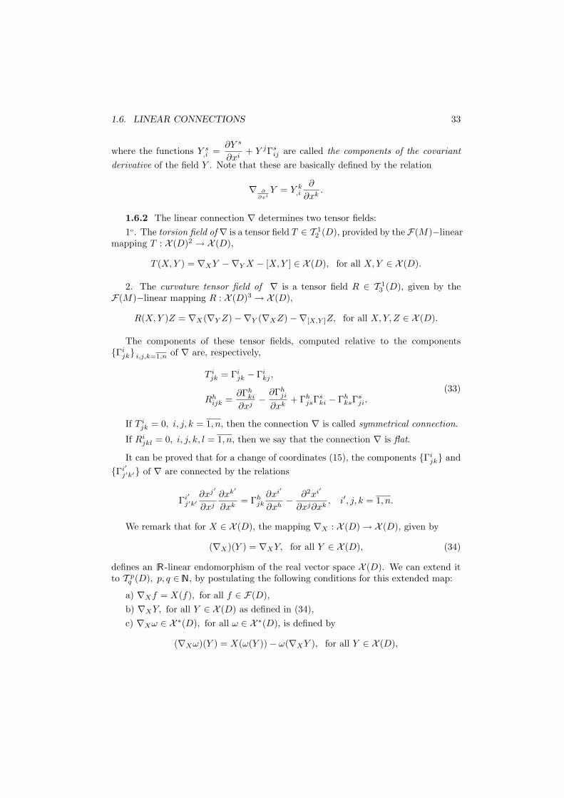
1.6. LINEAR CONNECTIONS 33
where the functions Y s,i =
∂Y s
∂xi+ Y jΓs
ij are called the components of the covariantderivative of the field Y . Note that these are basically defined by the relation
∇ ∂
∂xiY = Y k
,i
∂
∂xk.
1.6.2 The linear connection ∇ determines two tensor fields:1o. The torsion field of ∇ is a tensor field T ∈ T 1
2 (D), provided by the F(M)−linearmapping T : X (D)2 → X (D),
T (X,Y ) = ∇XY −∇Y X − [X,Y ] ∈ X (D), for all X, Y ∈ X (D).
2. The curvature tensor field of ∇ is a tensor field R ∈ T 13 (D), given by the
F(M)−linear mapping R : X (D)3 → X (D),
R(X, Y )Z = ∇X(∇Y Z)−∇Y (∇XZ)−∇[X,Y ]Z, for all X, Y, Z ∈ X (D).
The components of these tensor fields, computed relative to the componentsΓi
jk i,j,k=1,n of ∇ are, respectively,
T ijk = Γi
jk − Γikj ,
Rhijk =
∂Γhki
∂xj− ∂Γh
ji
∂xk+ Γh
jsΓski − Γh
ksΓsji.
(33)
If T ijk = 0, i, j, k = 1, n, then the connection ∇ is called symmetrical connection.
If Rijkl = 0, i, j, k, l = 1, n, then we say that the connection ∇ is flat.
It can be proved that for a change of coordinates (15), the components Γijk and
Γi′j′k′ of ∇ are connected by the relations
Γi′j′k′
∂xj′
∂xj
∂xk′
∂xk= Γh
jk
∂xi′
∂xh− ∂2xi′
∂xj∂xk, i′, j, k = 1, n.
We remark that for X ∈ X (D), the mapping ∇X : X (D) → X (D), given by
(∇X)(Y ) = ∇XY, for all Y ∈ X (D), (34)
defines an R -linear endomorphism of the real vector space X (D). We can extend itto T p
q (D), p, q ∈ N, by postulating the following conditions for this extended map:
a) ∇Xf = X(f), for all f ∈ F(D),b) ∇XY, for all Y ∈ X (D) as defined in (34),c) ∇Xω ∈ X ∗(D), for all ω ∈ X ∗(D), is defined by
(∇Xω)(Y ) = X(ω(Y ))− ω(∇XY ), for all Y ∈ X (D),
34 CHAPTER 1. TENSOR ALGEBRA AND ANALYSIS
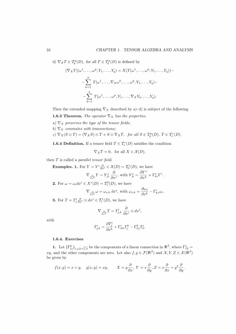
d) ∇XT ∈ T pq (D), for all T ∈ T p
q (D) is defined by
(∇XT )(ω1, . . . , ωp; Y1, . . . , Yq) = X(T (ω1, . . . , ωp; Y1, . . . , Yq))−
−p∑
k=1
T (ω1, . . . ,∇Xωk, . . . , ωp, Y1, . . . , Yq)−
−q∑
k=1
T (ω1, . . . , ωp, Y1, . . . ,∇XYk, . . . , Yq).
Then the extended mapping ∇X described by a)–d) is subject of the following
1.6.3 Theorem. The operator ∇X has the properties
a) ∇X preserves the type of the tensor fields;b) ∇X commutes with transvections;c) ∇X(S ⊗ T ) = (∇XS)⊗ T + S ⊗∇XT, for all S ∈ T p
q (D), T ∈ T rs (D).
1.6.4 Definition. If a tensor field T ∈ T rs (D) satisfies the condition
∇XT = 0, for all X ∈ X (D),
then T is called a parallel tensor field.
Examples. 1. For Y = Y i ∂∂xi ∈ X (D) = T 1
0 (D), we have
∇ ∂
∂xkY = Y s
,k
∂
∂xs, with Y s
,k =∂Y s
∂xk+ Γs
kiYi.
2. For ω = ωidxi ∈ X∗(D) = T 01 (D), we have
∇ ∂
∂xkω = ωs,k dxs, with ωs,k =
∂ωs
∂xk− Γi
ksωi.
3. For T = T ij
∂∂xi ⊗ dxj ∈ T 1
1 (D), we have
∇ ∂
∂xkT = T i
j,k
∂
∂xi⊗ dxj ,
with
T ij,k =
∂T ij
∂xk+ Γi
khThj − Γh
kjTih.
1.6.4. Exercises
1. Let Γkiji,j,k=1,n be the components of a linear connection in R2, where Γ1
12 =xy, and the other components are zero. Let also f, g ∈ F(R2) and X, Y, Z ∈ X (R2)be given by
f(x, y) = x + y, g(x, y) = xy, X = y∂
∂x, Y = x
∂
∂y, Z = x
∂
∂x+ y2 ∂
∂y.
1.6. LINEAR CONNECTIONS 35
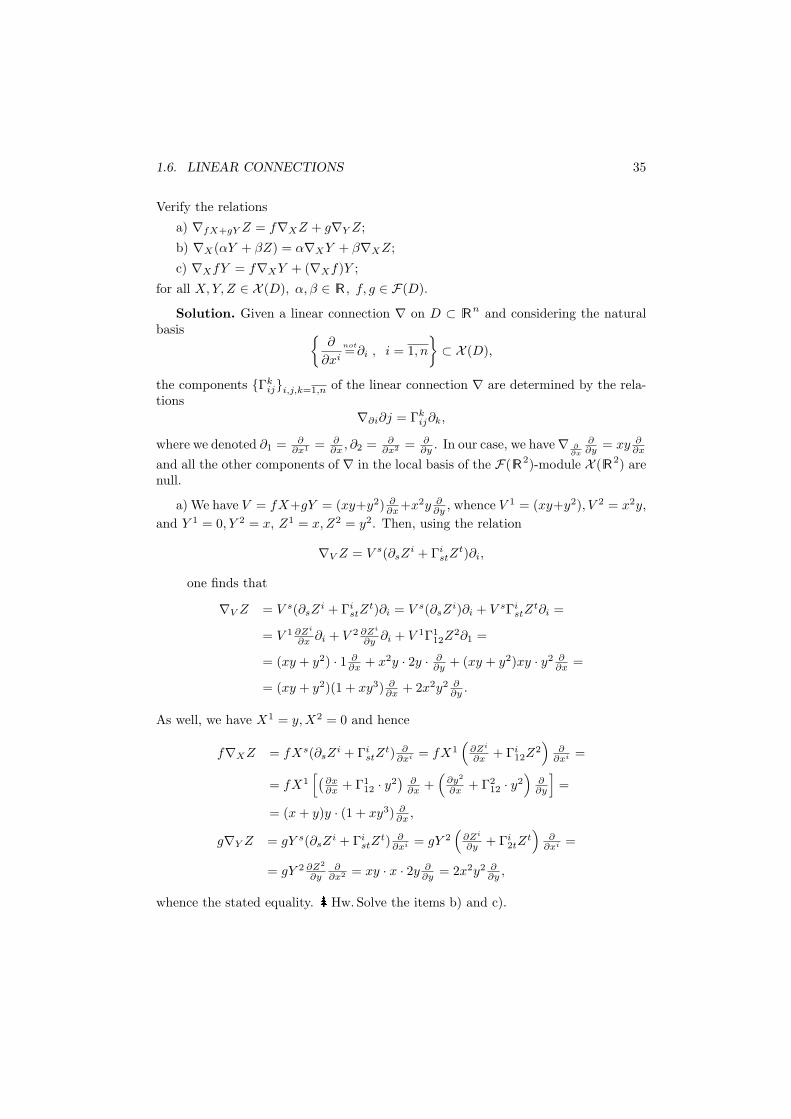
Verify the relations
a) ∇fX+gY Z = f∇XZ + g∇Y Z;
b) ∇X(αY + βZ) = α∇XY + β∇XZ;
c) ∇XfY = f∇XY + (∇Xf)Y ;
for all X, Y, Z ∈ X (D), α, β ∈ R , f, g ∈ F(D).
Solution. Given a linear connection ∇ on D ⊂ Rn and considering the naturalbasis
∂
∂xi
not=∂i , i = 1, n
⊂ X (D),
the components Γkiji,j,k=1,n of the linear connection ∇ are determined by the rela-
tions∇∂i∂j = Γk
ij∂k,
where we denoted ∂1 = ∂∂x1 = ∂
∂x , ∂2 = ∂∂x2 = ∂
∂y . In our case, we have∇ ∂∂x
∂∂y = xy ∂
∂x
and all the other components of ∇ in the local basis of the F( R2)-module X (R2) arenull.
a) We have V = fX+gY = (xy+y2) ∂∂x +x2y ∂
∂y , whence V 1 = (xy+y2), V 2 = x2y,and Y 1 = 0, Y 2 = x, Z1 = x,Z2 = y2. Then, using the relation
∇V Z = V s(∂sZi + Γi
stZt)∂i,
one finds that
∇V Z = V s(∂sZi + Γi
stZt)∂i = V s(∂sZ
i)∂i + V sΓistZ
t∂i =
= V 1 ∂Zi
∂x ∂i + V 2 ∂Zi
∂y ∂i + V 1Γ112Z
2∂1 =
= (xy + y2) · 1 ∂∂x + x2y · 2y · ∂
∂y + (xy + y2)xy · y2 ∂∂x =
= (xy + y2)(1 + xy3) ∂∂x + 2x2y2 ∂
∂y .
As well, we have X1 = y, X2 = 0 and hence
f∇XZ = fXs(∂sZi + Γi
stZt) ∂
∂xi = fX1(
∂Zi
∂x + Γi12Z
2)
∂∂xi =
= fX1[(
∂x∂x + Γ1
12 · y2)
∂∂x +
(∂y2
∂x + Γ212 · y2
)∂∂y
]=
= (x + y)y · (1 + xy3) ∂∂x ,
g∇Y Z = gY s(∂sZi + Γi
stZt) ∂
∂xi = gY 2(
∂Zi
∂y + Γi2tZ
t)
∂∂xi =
= gY 2 ∂Z2
∂y∂
∂x2 = xy · x · 2y ∂∂y = 2x2y2 ∂
∂y ,
whence the stated equality. Hw. Solve the items b) and c).
36 CHAPTER 1. TENSOR ALGEBRA AND ANALYSIS
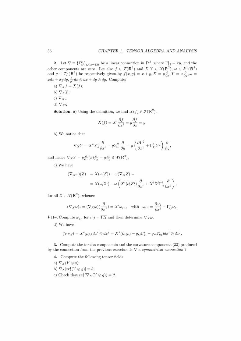
2. Let ∇ ≡ Γkiji,j,k=1,n be a linear connection in R2, where Γ1
12 = xy, and theother components are zero. Let also f ∈ F(R2) and X, Y ∈ X (R2), ω ∈ X ∗(R2)and g ∈ T 0
2 (R2) be respectively given by f(x, y) = x + y, X = y ∂∂x , Y = x ∂
∂y , ω =xdx + xydy, 1
y2 dx⊗ dx + dy ⊗ dy. Compute:
a) ∇Xf = X(f);b) ∇XY ;c) ∇Xω;d) ∇Xg.
Solution. a) Using the definition, we find X(f) ∈ F(R2),
X(f) = Xi ∂f
∂xi= y
∂f
∂x= y.
b) We notice that
∇XY = XkY i;k
∂
∂xi= yY 2
;1
∂
∂y= y
(∂Y 2
∂x1+ Γ2
1jYj
)∂
∂y,
and hence ∇XY = y ∂∂x (x) ∂
∂y = y ∂∂y ∈ X (R2).
c) We have
(∇Xω)(Z) = X(ω(Z))− ω(∇XZ) =
= X(ωiZi)− ω
(Xi(∂iZ
j)∂
∂xj+ XiZjΓk
ij
∂
∂xk
),
for all Z ∈ X (R2), whence
(∇Xω)j = (∇Xω)(∂
∂xj) = Xiωj;i, with ωj;i =
∂ωj
∂xi− Γs
ijωs.
Hw. Compute ωj;i for i, j = 1, 2 and then determine ∇Xω.
d) We have
(∇Xg) = Xkgij;kdxi ⊗ dxj = Xk(∂kgij − gsjΓski − gsiΓs
kj)dxi ⊗ dxj .
3. Compute the torsion components and the curvature components (33) producedby the connection from the previous exercise. Is ∇ a symmetrical connection ?
4. Compute the following tensor fieldsa) ∇X(Y ⊗ g);b) ∇X [tr1
2(Y ⊗ g)] ≡ θ;c) Check that tr1
2(∇X(Y ⊗ g)) = θ.
1.6. LINEAR CONNECTIONS 37
Hint. a) The tensor field U = Y ⊗ g ∈ T 12 (M) has the covariantly derived com-
ponentsU i
jk;l = ∂lUijk + Us
jkΓils − U i
skΓslj − U i
jsΓslk.
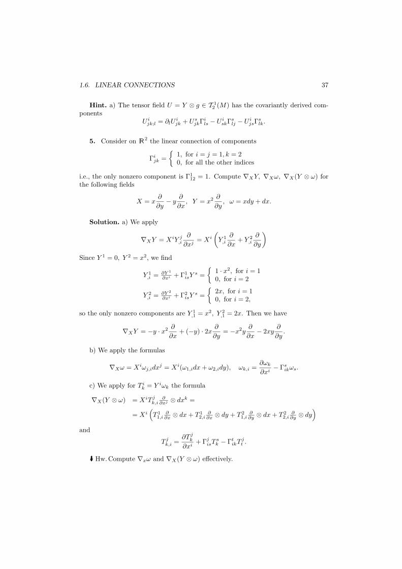
5. Consider on R2 the linear connection of components
Γijk =
1, for i = j = 1, k = 20, for all the other indices
i.e., the only nonzero component is Γ112 = 1. Compute ∇XY, ∇Xω, ∇X(Y ⊗ ω) for
the following fields
X = x∂
∂y− y
∂
∂x, Y = x2 ∂
∂y, ω = xdy + dx.
Solution. a) We apply
∇XY = XiY j,i
∂
∂xj= Xi
(Y 1
,i
∂
∂x+ Y 2
,i
∂
∂y
)
Since Y 1 = 0, Y 2 = x2, we find
Y 1,i = ∂Y 1
∂xi + Γ1isY
s =
1 · x2, for i = 10, for i = 2
Y 2,i = ∂Y 2
∂xi + Γ2isY
s =
2x, for i = 10, for i = 2,
so the only nonzero components are Y 1,1 = x2, Y 2
,1 = 2x. Then we have
∇XY = −y · x2 ∂
∂x+ (−y) · 2x
∂
∂y= −x2y
∂
∂x− 2xy
∂
∂y.
b) We apply the formulas
∇Xω = Xiωj,idxj = Xi(ω1,idx + ω2,idy), ωk,i =∂ωk
∂xi− Γs
ikωs.
c) We apply for T ik = Y iωk the formula
∇X(Y ⊗ ω) = XiT jk,i
∂∂xj ⊗ dxk =
= Xi(T 1
1,i∂∂x ⊗ dx + T 1
2,i∂∂x ⊗ dy + T 2
1,i∂∂y ⊗ dx + T 2
2,i∂∂y ⊗ dy
)
and
T jk,i =
∂T jk
∂xi+ Γj
isTsk − Γt
ikT jt .
Hw.Compute ∇xω and ∇X(Y ⊗ ω) effectively.
38 CHAPTER 1. TENSOR ALGEBRA AND ANALYSIS
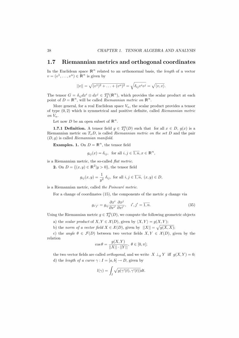
1.7 Riemannian metrics and orthogonal coordinates
In the Euclidean space Rn related to an orthonormal basis, the length of a vectorv = (v1, . . . , vn) ∈ Rn is given by
||v|| =√
(v1)2 + . . . + (vn)2 =√
δijvivj =√〈v, v〉.
The tensor G = δijdxi ⊗ dxj ∈ T 02 (Rn), which provides the scalar product at each
point of D = Rn, will be called Riemannian metric on Rn.More general, for a real Euclidean space Vn, the scalar product provides a tensor
of type (0, 2) which is symmetrical and positive definite, called Riemannian metricon Vn.
Let now D be an open subset of Rn.
1.7.1 Definition. A tensor field g ∈ T 02 (D) such that for all x ∈ D, g(x) is a
Riemannian metric on TxD, is called Riemannian metric on the set D and the pair(D, g) is called Riemannian manifold.
Examples. 1. On D = Rn, the tensor field
gij(x) = δij , for all i, j ∈ 1, n, x ∈ Rn,
is a Riemannian metric, the so-called flat metric.2. On D = (x, y) ∈ R2|y > 0, the tensor field
gij(x, y) =1y2
δij , for all i, j ∈ 1, n, (x, y) ∈ D,
is a Riemannian metric, called the Poincare metric.
For a change of coordinates (15), the components of the metric g change via
gi′j′ = gij∂xi
∂xi′∂xj
∂xj′ , i′, j′ = 1, n. (35)
Using the Riemannian metric g ∈ T 02 (D), we compute the following geometric objects
a) the scalar product of X, Y ∈ X (D), given by 〈X,Y 〉 = g(X, Y );b) the norm of a vector field X ∈ X (D), given by ||X|| =
√g(X,X);
c) the angle θ ∈ F(D) between two vector fields X, Y ∈ X (D), given by therelation
cos θ =g(X, Y )||X|| · ||Y || , θ ∈ [0, π];
the two vector fields are called orthogonal, and we write X ⊥g Y iff g(X,Y ) = 0;d) the length of a curve γ : I = [a, b] → D, given by
l(γ) =∫
I
√g(γ′(t), γ′(t))dt.
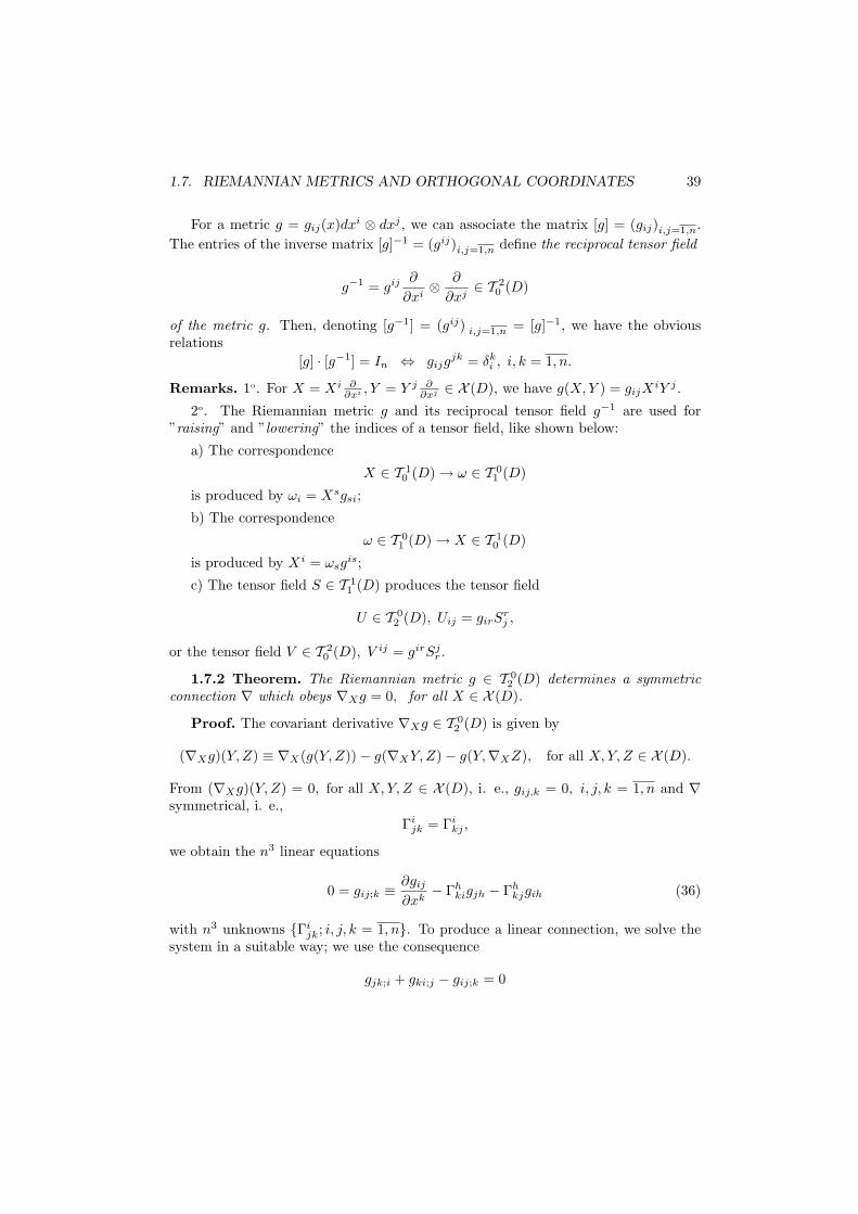
1.7. RIEMANNIAN METRICS AND ORTHOGONAL COORDINATES 39
For a metric g = gij(x)dxi ⊗ dxj , we can associate the matrix [g] = (gij)i,j=1,n.The entries of the inverse matrix [g]−1 = (gij)i,j=1,n define the reciprocal tensor field
g−1 = gij ∂
∂xi⊗ ∂
∂xj∈ T 2
0 (D)
of the metric g. Then, denoting [g−1] = (gij) i,j=1,n = [g]−1, we have the obviousrelations
[g] · [g−1] = In ⇔ gijgjk = δk
i , i, k = 1, n.
Remarks. 1o. For X = Xi ∂∂xi , Y = Y j ∂
∂xj ∈ X (D), we have g(X, Y ) = gijXiY j .
2o. The Riemannian metric g and its reciprocal tensor field g−1 are used for”raising” and ”lowering” the indices of a tensor field, like shown below:
a) The correspondence
X ∈ T 10 (D) → ω ∈ T 0
1 (D)
is produced by ωi = Xsgsi;
b) The correspondence
ω ∈ T 01 (D) → X ∈ T 1
0 (D)
is produced by Xi = ωsgis;
c) The tensor field S ∈ T 11 (D) produces the tensor field
U ∈ T 02 (D), Uij = girS
rj ,
or the tensor field V ∈ T 20 (D), V ij = girSj
r .
1.7.2 Theorem. The Riemannian metric g ∈ T 02 (D) determines a symmetric
connection ∇ which obeys ∇Xg = 0, for all X ∈ X (D).
Proof. The covariant derivative ∇Xg ∈ T 02 (D) is given by
(∇Xg)(Y, Z) ≡ ∇X(g(Y, Z))− g(∇XY,Z)− g(Y,∇XZ), for all X, Y, Z ∈ X (D).
From (∇Xg)(Y, Z) = 0, for all X, Y, Z ∈ X (D), i. e., gij,k = 0, i, j, k = 1, n and ∇symmetrical, i. e.,
Γijk = Γi
kj ,
we obtain the n3 linear equations
0 = gij;k ≡ ∂gij
∂xk− Γh
kigjh − Γhkjgih (36)
with n3 unknowns Γijk; i, j, k = 1, n. To produce a linear connection, we solve the
system in a suitable way; we use the consequence
gjk;i + gki;j − gij;k = 0
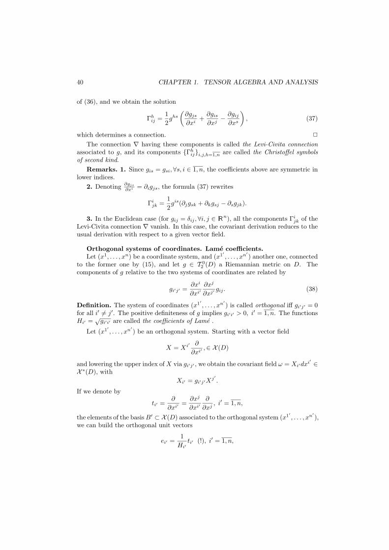
40 CHAPTER 1. TENSOR ALGEBRA AND ANALYSIS
of (36), and we obtain the solution
Γhij =
12ghs
(∂gjs
∂xi+
∂gis
∂xj− ∂gij
∂xs
), (37)
which determines a connection. 2
The connection ∇ having these components is called the Levi-Civita connectionassociated to g, and its components Γh
iji,j,h=1,n are called the Christoffel symbolsof second kind.
Remarks. 1. Since gis = gsi,∀s, i ∈ 1, n, the coefficients above are symmetric inlower indices.
2. Denoting ∂gjs
∂xi = ∂igjs, the formula (37) rewrites
Γijk =
12gis(∂jgsk + ∂kgsj − ∂sgjk).
3. In the Euclidean case (for gij = δij , ∀i, j ∈ Rn), all the components Γijk of the
Levi-Civita connection ∇ vanish. In this case, the covariant derivation reduces to theusual derivation with respect to a given vector field.
Orthogonal systems of coordinates. Lame coefficients.Let (x1, . . . , xn) be a coordinate system, and (x1′ , . . . , xn′) another one, connected
to the former one by (15), and let g ∈ T 02 (D) a Riemannian metric on D. The
components of g relative to the two systems of coordinates are related by
gi′j′ =∂xi
∂xi′∂xj
∂xj′ gij . (38)
Definition. The system of coordinates (x1′ , . . . , xn′) is called orthogonal iff gi′j′ = 0for all i′ 6= j′. The positive definiteness of g implies gi′i′ > 0, i′ = 1, n. The functionsHi′ =
√gi′i′ are called the coefficients of Lame .
Let (x1′ , . . . , xn′) be an orthogonal system. Starting with a vector field
X = Xi′ ∂
∂xi′ ,∈ X (D)
and lowering the upper index of X via gi′j′ , we obtain the covariant field ω = Xi′dxi′ ∈X ∗(D), with
Xi′ = gi′j′Xj′ .
If we denote by
ti′ =∂
∂xi′ =∂xj
∂xi′∂
∂xj, i′ = 1, n,
the elements of the basis B′ ⊂ X (D) associated to the orthogonal system (x1′ , . . . , xn′),we can build the orthogonal unit vectors
ei′ =1
Hi′ti′ (!), i′ = 1, n,
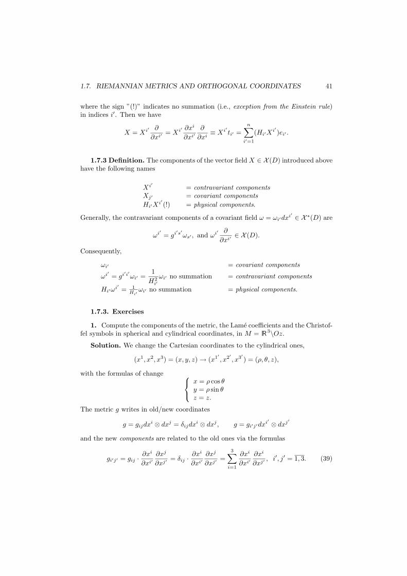
1.7. RIEMANNIAN METRICS AND ORTHOGONAL COORDINATES 41
where the sign ”(!)” indicates no summation (i.e., exception from the Einstein rule)in indices i′. Then we have
X = Xi′ ∂
∂xi′ = Xi′ ∂xi
∂xi′∂
∂xi≡ Xi′ti′ =
n∑
i′=1
(Hi′Xi′)ei′ .
1.7.3 Definition. The components of the vector field X ∈ X (D) introduced abovehave the following names
Xi′ = contravariant componentsXj′ = covariant componentsHi′X
i′(!) = physical components.
Generally, the contravariant components of a covariant field ω = ωi′dxi′ ∈ X ∗(D) are
ωi′ = gi′s′ωs′ , and ωi′ ∂
∂xi′ ∈ X (D).
Consequently,
ωi′ = covariant components
ωi′ = gi′i′ωi′ =1
H2i′
ωi′ no summation = contravariant components
Hi′ωi′ = 1
Hi′ωi′ no summation = physical components.
1.7.3. Exercises
1. Compute the components of the metric, the Lame coefficients and the Christof-fel symbols in spherical and cylindrical coordinates, in M = R3\Oz.
Solution. We change the Cartesian coordinates to the cylindrical ones,
(x1, x2, x3) = (x, y, z) → (x1′ , x2′ , x3′) = (ρ, θ, z),
with the formulas of change
x = ρ cos θy = ρ sin θz = z.
The metric g writes in old/new coordinates
g = gijdxi ⊗ dxj = δijdxi ⊗ dxj , g = gi′j′dxi′ ⊗ dxj′
and the new components are related to the old ones via the formulas
gi′j′ = gij · ∂xi
∂xi′∂xj
∂xj′ = δij · ∂xi
∂xi′∂xj
∂xj′ =3∑
i=1
∂xi
∂xi′∂xi
∂xj′ , i′, j′ = 1, 3. (39)
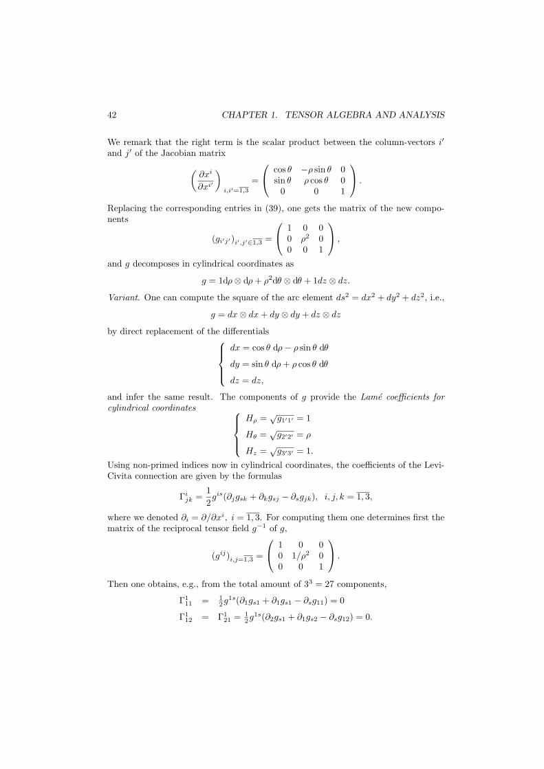
42 CHAPTER 1. TENSOR ALGEBRA AND ANALYSIS
We remark that the right term is the scalar product between the column-vectors i′
and j′ of the Jacobian matrix
(∂xi
∂xi′
)
i,i′=1,3
=
cos θ −ρ sin θ 0sin θ ρ cos θ 0
0 0 1
.
Replacing the corresponding entries in (39), one gets the matrix of the new compo-nents
(gi′j′)i′,j′∈1,3 =
1 0 00 ρ2 00 0 1
,
and g decomposes in cylindrical coordinates as
g = 1dρ⊗ dρ + ρ2dθ ⊗ dθ + 1dz ⊗ dz.
Variant. One can compute the square of the arc element ds2 = dx2 + dy2 + dz2, i.e.,
g = dx⊗ dx + dy ⊗ dy + dz ⊗ dz
by direct replacement of the differentials
dx = cos θ dρ− ρ sin θ dθ
dy = sin θ dρ + ρ cos θ dθ
dz = dz,
and infer the same result. The components of g provide the Lame coefficients forcylindrical coordinates
Hρ =√
g1′1′ = 1
Hθ =√
g2′2′ = ρ
Hz =√
g3′3′ = 1.
Using non-primed indices now in cylindrical coordinates, the coefficients of the Levi-Civita connection are given by the formulas
Γijk =
12gis(∂jgsk + ∂kgsj − ∂sgjk), i, j, k = 1, 3,
where we denoted ∂i = ∂/∂xi, i = 1, 3. For computing them one determines first thematrix of the reciprocal tensor field g−1 of g,
(gij)i,j=1,3 =
1 0 00 1/ρ2 00 0 1
.
Then one obtains, e.g., from the total amount of 33 = 27 components,
Γ111 = 1
2g1s(∂1gs1 + ∂1gs1 − ∂sg11) = 0
Γ112 = Γ1
21 = 12g1s(∂2gs1 + ∂1gs2 − ∂sg12) = 0.
1.8. DIFFERENTIAL OPERATORS 43
1.8 Differential operators
Let D ⊂ R3 be an open and connected set and δij , i, j = 1, 2, 3, be the Riemannianmetric on D. We shall implicitly use the Cartesian coordinates on D.
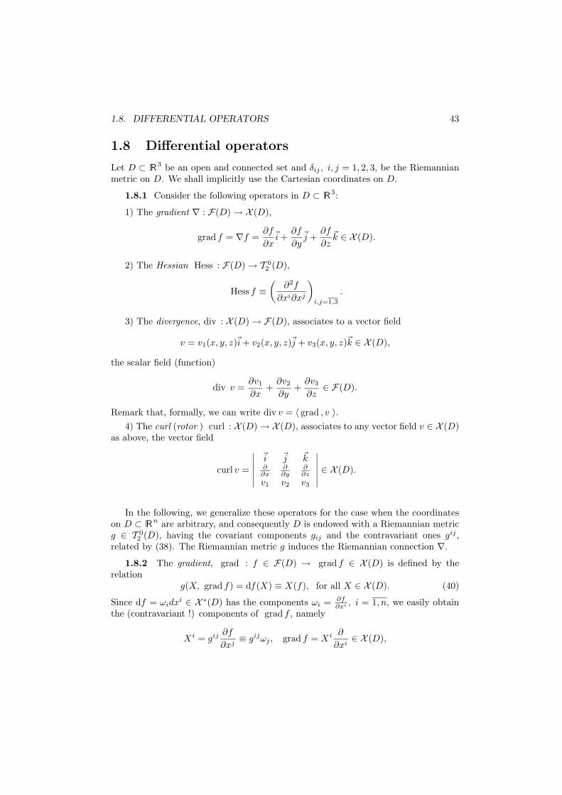
1.8.1 Consider the following operators in D ⊂ R3:
1) The gradient ∇ : F(D) → X (D),
grad f = ∇f =∂f
∂x~i +
∂f
∂y~j +
∂f
∂z~k ∈ X (D).
2) The Hessian Hess : F(D) → T 02 (D),
Hess f ≡(
∂2f
∂xi∂xj
)
i,j=1,3
.
3) The divergence, div : X (D) → F(D), associates to a vector field
v = v1(x, y, z)~i + v2(x, y, z)~j + v3(x, y, z)~k ∈ X (D),
the scalar field (function)
div v =∂v1
∂x+
∂v2
∂y+
∂v3
∂z∈ F(D).
Remark that, formally, we can write div v = 〈 grad , v 〉.4) The curl (rotor ) curl : X (D) → X (D), associates to any vector field v ∈ X (D)
as above, the vector field
curl v =
∣∣∣∣∣∣
~i ~j ~k∂∂x
∂∂y
∂∂z
v1 v2 v3
∣∣∣∣∣∣∈ X (D).
In the following, we generalize these operators for the case when the coordinateson D ⊂ Rn are arbitrary, and consequently D is endowed with a Riemannian metricg ∈ T 0
2 (D), having the covariant components gij and the contravariant ones gij ,related by (38). The Riemannian metric g induces the Riemannian connection ∇.
1.8.2 The gradient, grad : f ∈ F(D) → grad f ∈ X (D) is defined by therelation
g(X, grad f) = df(X) ≡ X(f), for all X ∈ X (D). (40)
Since df = ωidxi ∈ X ∗(D) has the components ωi = ∂f∂xi , i = 1, n, we easily obtain
the (contravariant !) components of grad f , namely
Xi = gij ∂f
∂xj≡ gijωj , grad f = Xi ∂
∂xi∈ X (D),
44 CHAPTER 1. TENSOR ALGEBRA AND ANALYSIS
so that
grad f =(
gij ∂f
∂xj
)∂
∂xi∈ X (D).
This operator has the following properties
a) grad (a1f1 + a2f2) = a1 grad f1 + a2 grad f2;
b) grad(
f1
f2
)=
1f22
[f2 grad f1 − f1 grad f2];
c) grad ϕ(f) = (ϕ′ f) grad f ,
for all a1,2 ∈ R , f, f1, f2 ∈ F(D), ϕ ∈ C∞(R).
Remarks. 1o. Sometimes, instead of the symbol ”grad” we shall use ∇ (nabla).
2o.The solutions of the system
∂f
∂xi= 0, i ∈ 1, n,
give the critical points of f ∈ F(D). The system can be briefly rewritten in the form
grad f = 0.
Theorem. If f has no critical points, then
a) grad f is orthogonal to the hypersurfaces described by f(x) = k, (k ∈ R), whichare called constant level sets;
b) grad f shows at each point the sense and direction of the steepest (highest)increase of the function f .
Proof. We prove a). Let Σ : f(x) = c, c ∈ R arbitrary and fixed. Consider thecoordinates x = (x1, . . . , xn) ∈ Rn, and a curve on Σ,
α : I ⊂ R → Σ ⊂ Rn,
given by α(t) = (x1(t), . . . , xn(t)), t ∈ I. Then
f(α(t)) = f(x1(t), . . . , xn(t)) = c, for all t ∈ I. (41)
Differentiating (41) by t and considering the relations
grad f = gij ∂f
∂xj
∂
∂xiand α′ =
(dx1
dt, . . . ,
dxn
dt
),
we infer that∂f
∂xi
dxi
dt= 0 ⇔ g( grad f, α′) = 0.
1.8. DIFFERENTIAL OPERATORS 45
Indeed
g( grad f, α′) = grs
(gri ∂f
∂xi
)dxs
dt= δi
s
∂f
∂xi
dxs
dt=
∂f
∂xi
dxi
dt= 0,
and hence grad f ⊥g α′. 2
1.8.3 Let ∇ be the Riemannian connection on D. The Hessian is the operatorHess : F(D) → T 0
2 (D), which associates to any function f ∈ F(D), a (0, 2)-typetensor, given by Hess f = ∇(df), i.e.,
Hess f(X, Y ) = (∇X df)(Y ), , for all X, Y ∈ X (D).
In coordinates,Hess f = ( Hess f)jk dxj ⊗ dxk (42)
with the components
( Hess f)jk =∂2f
∂xj∂xk− Γh
jk
∂f
∂xh, j, k = 1, n, (43)
where Γijk are the Christoffel symbols of g. The tensor field Hess f is called the
Hessian of f . The operator Hess is intensively used in the theory of extrema.
1.8.4 The divergence is the operator div : X (D) → F(D), given by
div X = Xi,i =
∂Xi
∂xi+ Γi
ikXk, for all X = Xi ∂
∂xi∈ X (D). (44)
We remind that Xi,j = ∂Xi
∂xj + ΓijkXk, and that the sum about i above means the
transvection tr11 of the (1, 1)-type field T = Xi
,j∂
∂xi ⊗ dxj ∈ T 11 (D).
Proposition. Denoting G = det (gij), an equivalent expression for divX is
divX =1√G
∂
∂xi(√
GXi), for all X ∈ X (D).
Proof. By direct computation, we obtain
Γiij =
12gik
(∂gjk
∂xi+
∂gik
∂xj− ∂gij
∂xk
)=
12gik ∂gik
∂xj, (45)
and the partial derivative of the determinant G can be written
∂G
∂xj=
∂G
∂gik
∂gik
∂xj= Ggik · ∂gik
∂xj. (46)
Using (46), the relation (45) becomes
Γiij =
12G
∂G
∂xj=
1√G
∂√
G
∂xj,
46 CHAPTER 1. TENSOR ALGEBRA AND ANALYSIS
and, replacing in the formula (44), we infer
divX = Xi,i =
∂Xi
∂xi+
1√G
(∂√
G
∂xk
)Xk =
1√G
(√G
∂Xi
∂xi+ Xi ∂
√G
∂xi
),
whence the statement holds true. 2
Remarks. The divergence has the following properties1) div (fX) = X(f) + fdiv X;2) div (aX + bY ) = a div X + b div Y, for all a, b ∈ R , X, Y ∈ X (D), f ∈ F(D).
1.8.5 Definitions. a) The Laplacian is the operator ∆ : F(D) → F(D), given by
∆f = div ( grad f), for all f ∈ F(D).
In coordinates, it has the expression
∆f =1√G
∂
∂xl
(√Ggkl ∂f
∂xk
)= gklfkl,
where fklk,l=1,n are the components of the Hessian (43).
b) A function f ∈ F(D) which obeys ∆f = 0 is called harmonic.
1.8.6 Definition. The curl (rotor ) is the operator curl : X (D) → T 02 (D), given
bycurl X = (ωj;i − ωi;j) dxi ⊗ dxj ∈ T 0
2 (D), for all X ∈ X (D),
with ωj = gjsXs, i.e., the 1-form ω = ωjdxj ∈ X ∗(D) is obtained from X by lowering
the index and ωj;i = ∂ωj
∂xi −Γkijωk, i, j = 1, n, where Γk
ij are the Christoffel symbols ofg. In the Euclidean case, when gij = δij , we have
curl X =(
∂
∂xiXj − ∂
∂xjXi
)dxi ⊗ dxj , for all X ∈ X (D).
Remarks. 1o. The tensor curl X ∈ T 02 (D) is antisymmetrical in lower indices
(i.e., denoting the components by aij , we have aij = −aji, for all i, j = 1, n).2o. In the case D ⊂ R3, we can attach to curl X a contravariant vector field,
namely
( curl X)i =1√G
(∂
∂xj(gksX
s)− ∂
∂xk(gjsX
s))
,
where the triple i, j, k is a cyclic permutation of the numbers 1, 2, 3.3o. For D ⊂ R3, to curl X we can associate the (antisymmetrical) matrix of the
form
[ curl X] =
0 a12 a13
−a12 0 a23
−a13 −a23 0
.
1.8. DIFFERENTIAL OPERATORS 47
1.8.7 Let us change the Cartesian coordinates (x, y, z) to the orthogonal coor-dinates (u, v, w), via the formulas
x = x(u, v, w)y = y(u, v, w)z = z(u, v, w).
Fix a point P (x0, y0, z0) ∈ R3,
x0 = x(u0, v0, w0)y0 = y(u0, v0, w0)z0 = z(u0, v0, w0).
Consider the three coordinate lines and the three coordinate surfaces through thispoint; for example, the (u)-line is given parametrically by
x = x(u, v0, w0)y = y(u, v0, w0)z = z(u, v0, w0)
and the u = u0 surface is given parametrically by
x = x(u0, v, w)y = y(u0, v, w)z = z(u0, v, w).
We suppose that the new system is orthogonal (i.e., the tangents to the coordinatelines are mutually orthogonal).
Let ~r = x(u, v, w)~i+y(u, v, w)~j +z(u, v, w)~k be the position vector and the partialderivatives
~ru =∂~r
∂u, ~rv =
∂~r
∂v, ~rw =
∂~r
∂w.
These vectors are mutually orthogonal, and the Lame coefficients of the new coordi-nate system are the norms
Hu = ||~ru||, Hv = ||~rv||, Hw = ||~rw||,
and one can normalize the family of these vectors, obtaining the orthonormal basis~eu, ~ev, ~ew ⊂ X (R3) given by
~eu =1
Hu~ru, ~ev =
1Hv
~rv, ~ew =1
Hw~rw.
The area element in the plane x = x0, expressed in Cartesian coordinates is
dσ = dy ∧ dznot= dy dz,
48 CHAPTER 1. TENSOR ALGEBRA AND ANALYSIS
and the area element on the curvilinear surface u = u0 is given by
dσ = Hv Hwdv ∧ dwnot= Hv Hw dv dw.
Also, the volume element in the Cartesian system is
dV = dx ∧ dy ∧ dznot= dx dy dz
and in curvilinear coordinates,
dV = HuHvHw du ∧ dv ∧ dwnot= HuHvHw du dv dw.
1.8.8 Let D ⊂ R3. We pass from the Cartesian coordinates (x1, x2, x3) =(x, y, z). We pass to a general orthogonal system of coordinates (x1′ , x2′ , x3′) =(u, v, w).
The gradient
grad f =∂f
∂x~i +
∂f
∂y~j +
∂f
∂z~k ∈ X (D)
rewritesgrad f =
1Hu
∂f
∂u~eu +
1Hv
∂f
∂v~ev +
1Hw
∂f
∂w~ew = S
uvw
1Hu
∂f
∂u~eu, (47)
where the coefficients of the linear combination above are the physical components ofgrad f .
Also, in physical components, we have
~V = Vu~eu + Vv~ev + Vw~ew ∈ X (D), D ⊂ R3;
the rotor and the divergence of the vector field ~V rewrite
curl ~V =1
HuHvHw
∣∣∣∣∣∣∣∣
Hu~eu Hv~ev Hw~ew
∂∂u
∂∂v
∂∂w
HuVu HvVv HwVw
∣∣∣∣∣∣∣∣
div ~V =1
HuHvHw
[∂
∂u(VuHvHw) +
∂
∂v(VvHwHu) +
∂
∂w(VwHuHv)
]=
=1H
Suvw
∂
∂u(VuHvHw),
(48)
where H = HuHvHw. Moreover, since ∆f = div ( grad f), for all f ∈ F(D), replac-ing ~V with grad f , we obtain the expression of the Laplacian of f ,
∆f =1
HuHvHw
[∂
∂u
(∂f
∂u
HvHw
Hu
)+
∂
∂v
(∂f
∂v
HwHu
Hv
)+
∂
∂w
(∂f
∂w
HuHv
Hw
)]=
=1H
Suvw
∂
∂u
(∂f
∂u
HvHw
Hu
).
(49)
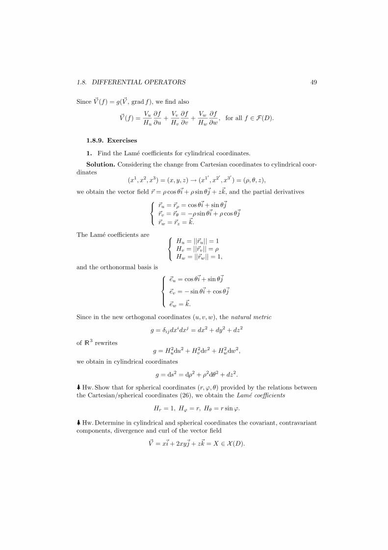
1.8. DIFFERENTIAL OPERATORS 49
Since ~V (f) = g(~V , grad f), we find also
~V (f) =Vu
Hu
∂f
∂u+
Vv
Hv
∂f
∂v+
Vw
Hw
∂f
∂w, for all f ∈ F(D).
1.8.9. Exercises
1. Find the Lame coefficients for cylindrical coordinates.
Solution. Considering the change from Cartesian coordinates to cylindrical coor-dinates
(x1, x2, x3) = (x, y, z) → (x1′ , x2′ , x3′) = (ρ, θ, z),
we obtain the vector field ~r = ρ cos θ~i + ρ sin θ~j + z~k, and the partial derivatives
~ru = ~rρ = cos θ~i + sin θ~j
~rv = ~rθ = −ρ sin θ~i + ρ cos θ~j
~rw = ~rz = ~k.
The Lame coefficients are
Hu = ||~ru|| = 1Hv = ||~rv|| = ρHw = ||~rw|| = 1,
and the orthonormal basis is
~eu = cos θ~i + sin θ~j
~ev = − sin θ~i + cos θ~j
~ew = ~k.
Since in the new orthogonal coordinates (u, v, w), the natural metric
g = δijdxidxj = dx2 + dy2 + dz2
of R3 rewritesg = H2
udu2 + H2vdv2 + H2
wdw2,
we obtain in cylindrical coordinates
g = ds2 = dρ2 + ρ2dθ2 + dz2.
Hw. Show that for spherical coordinates (r, ϕ, θ) provided by the relations betweenthe Cartesian/spherical coordinates (26), we obtain the Lame coefficients
Hr = 1, Hϕ = r, Hθ = r sin ϕ.
Hw. Determine in cylindrical and spherical coordinates the covariant, contravariantcomponents, divergence and curl of the vector field
~V = x~i + 2xy~j + z~k = X ∈ X (D).
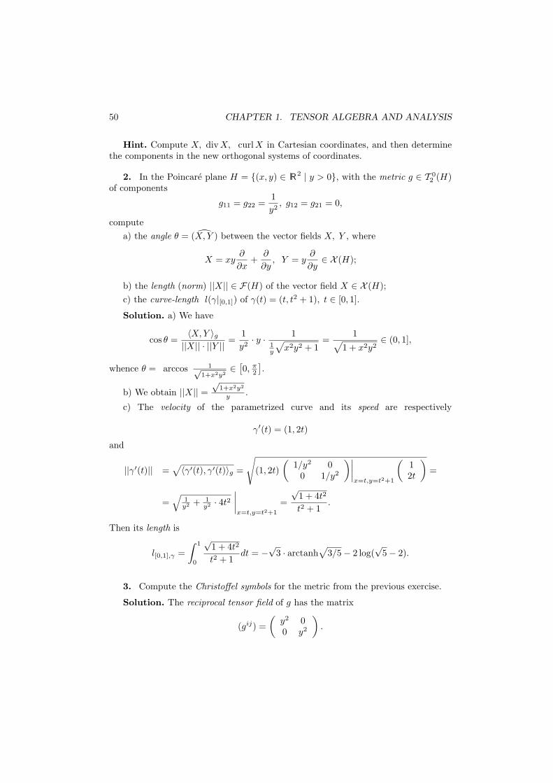
50 CHAPTER 1. TENSOR ALGEBRA AND ANALYSIS
Hint. Compute X, div X, curl X in Cartesian coordinates, and then determinethe components in the new orthogonal systems of coordinates.
2. In the Poincare plane H = (x, y) ∈ R2 | y > 0, with the metric g ∈ T 02 (H)
of components
g11 = g22 =1y2
, g12 = g21 = 0,
computea) the angle θ = (X, Y ) between the vector fields X, Y , where
X = xy∂
∂x+
∂
∂y, Y = y
∂
∂y∈ X (H);
b) the length (norm) ||X|| ∈ F(H) of the vector field X ∈ X (H);c) the curve-length l(γ|[0,1]) of γ(t) = (t, t2 + 1), t ∈ [0, 1].
Solution. a) We have
cos θ =〈X, Y 〉g||X|| · ||Y || =
1y2· y · 1
1y
√x2y2 + 1
=1√
1 + x2y2∈ (0, 1],
whence θ = arccos 1√1+x2y2
∈ [0, π
2
].
b) We obtain ||X|| =√
1+x2y2
y .
c) The velocity of the parametrized curve and its speed are respectively
γ′(t) = (1, 2t)
and
||γ′(t)|| =√〈γ′(t), γ′(t)〉g =
√(1, 2t)
(1/y2 0
0 1/y2
)∣∣∣∣x=t,y=t2+1
(12t
)=
=√
1y2 + 1
y2 · 4t2∣∣∣∣x=t,y=t2+1
=√
1 + 4t2
t2 + 1.
Then its length is
l[0,1],γ =∫ 1
0
√1 + 4t2
t2 + 1dt = −
√3 · arctanh
√3/5− 2 log(
√5− 2).
3. Compute the Christoffel symbols for the metric from the previous exercise.
Solution. The reciprocal tensor field of g has the matrix
(gij) =(
y2 00 y2
).
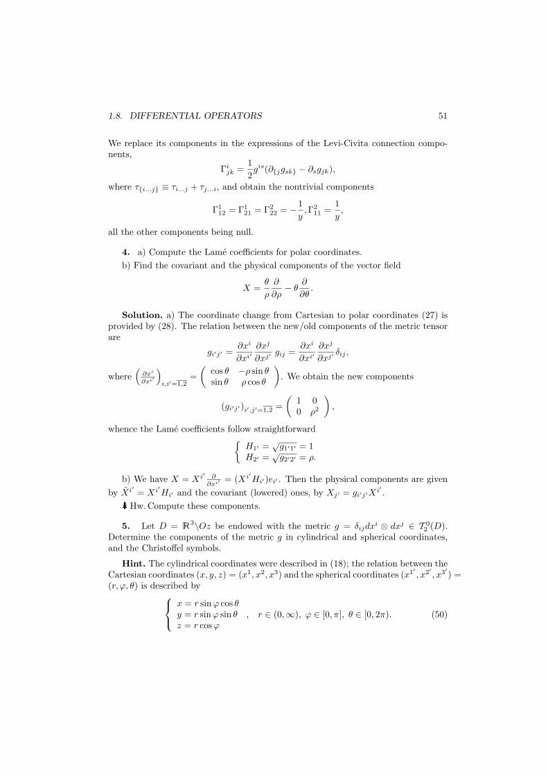
1.8. DIFFERENTIAL OPERATORS 51
We replace its components in the expressions of the Levi-Civita connection compo-nents,
Γijk =
12gis(∂jgsk − ∂sgjk),
where τi...j ≡ τi...j + τj...i, and obtain the nontrivial components
Γ112 = Γ1
21 = Γ222 = −1
y, Γ2
11 =1y,
all the other components being null.
4. a) Compute the Lame coefficients for polar coordinates.b) Find the covariant and the physical components of the vector field
X =θ
ρ
∂
∂ρ− θ
∂
∂θ.
Solution. a) The coordinate change from Cartesian to polar coordinates (27) isprovided by (28). The relation between the new/old components of the metric tensorare
gi′j′ =∂xi
∂xi′∂xj
∂xj′ gij =∂xi
∂xi′∂xj
∂xj′ δij ,
where(
∂xi
∂xi′
)i,i′=1,2
=(
cos θ −ρ sin θsin θ ρ cos θ
). We obtain the new components
(gi′j′)i′,j′=1,2 =(
1 00 ρ2
),
whence the Lame coefficients follow straightforward
H1′ =√
g1′1′ = 1H2′ =
√g2′2′ = ρ.
b) We have X = Xi′ ∂∂xi′ = (Xi′Hi′)ei′ . Then the physical components are given
by Xi′ = Xi′Hi′ and the covariant (lowered) ones, by Xj′ = gi′j′Xi′ .
Hw.Compute these components.
5. Let D = R3\Oz be endowed with the metric g = δijdxi ⊗ dxj ∈ T 02 (D).
Determine the components of the metric g in cylindrical and spherical coordinates,and the Christoffel symbols.
Hint. The cylindrical coordinates were described in (18); the relation between theCartesian coordinates (x, y, z) = (x1, x2, x3) and the spherical coordinates (x1′ , x2′ , x3′) =(r, ϕ, θ) is described by
x = r sin ϕ cos θy = r sin ϕ sin θz = r cos ϕ
, r ∈ (0,∞), ϕ ∈ [0, π], θ ∈ [0, 2π). (50)
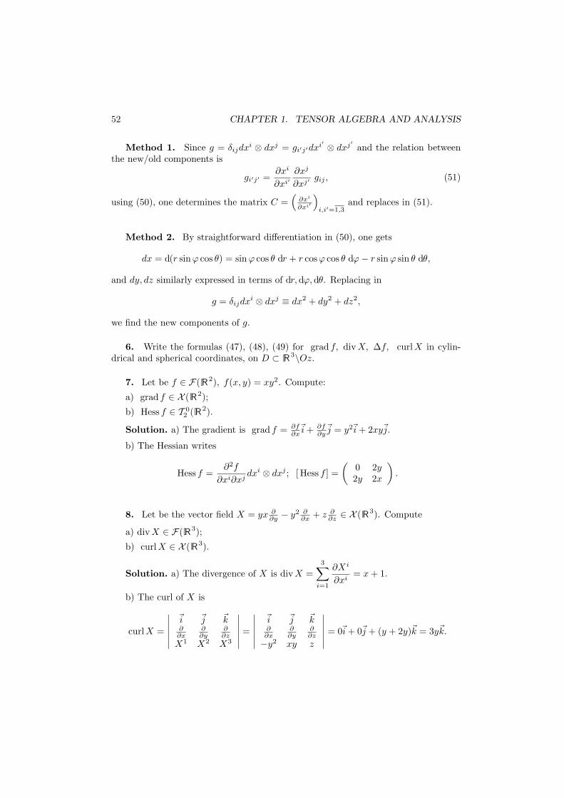
52 CHAPTER 1. TENSOR ALGEBRA AND ANALYSIS
Method 1. Since g = δijdxi ⊗ dxj = gi′j′dxi′ ⊗ dxj′ and the relation betweenthe new/old components is
gi′j′ =∂xi
∂xi′∂xj
∂xj′ gij , (51)
using (50), one determines the matrix C =(
∂xi
∂xi′
)i,i′=1,3
and replaces in (51).
Method 2. By straightforward differentiation in (50), one gets
dx = d(r sin ϕ cos θ) = sin ϕ cos θ dr + r cos ϕ cos θ dϕ− r sin ϕ sin θ dθ,
and dy, dz similarly expressed in terms of dr,dϕ, dθ. Replacing in
g = δijdxi ⊗ dxj ≡ dx2 + dy2 + dz2,
we find the new components of g.
6. Write the formulas (47), (48), (49) for grad f, divX, ∆f, curlX in cylin-drical and spherical coordinates, on D ⊂ R3\Oz.
7. Let be f ∈ F(R2), f(x, y) = xy2. Compute:
a) grad f ∈ X ( R2);
b) Hess f ∈ T 02 (R2).
Solution. a) The gradient is grad f = ∂f∂x
~i + ∂f∂y
~j = y2~i + 2xy~j.
b) The Hessian writes
Hess f =∂2f
∂xi∂xjdxi ⊗ dxj ; [ Hess f ] =
(0 2y2y 2x
).
8. Let be the vector field X = yx ∂∂y − y2 ∂
∂x + z ∂∂z ∈ X (R3). Compute
a) div X ∈ F(R3);
b) curl X ∈ X ( R3).
Solution. a) The divergence of X is div X =3∑
i=1
∂Xi
∂xi= x + 1.
b) The curl of X is
curl X =
∣∣∣∣∣∣
~i ~j ~k∂∂x
∂∂y
∂∂z
X1 X2 X3
∣∣∣∣∣∣=
∣∣∣∣∣∣
~i ~j ~k∂∂x
∂∂y
∂∂z
−y2 xy z
∣∣∣∣∣∣= 0~i + 0~j + (y + 2y)~k = 3y~k.
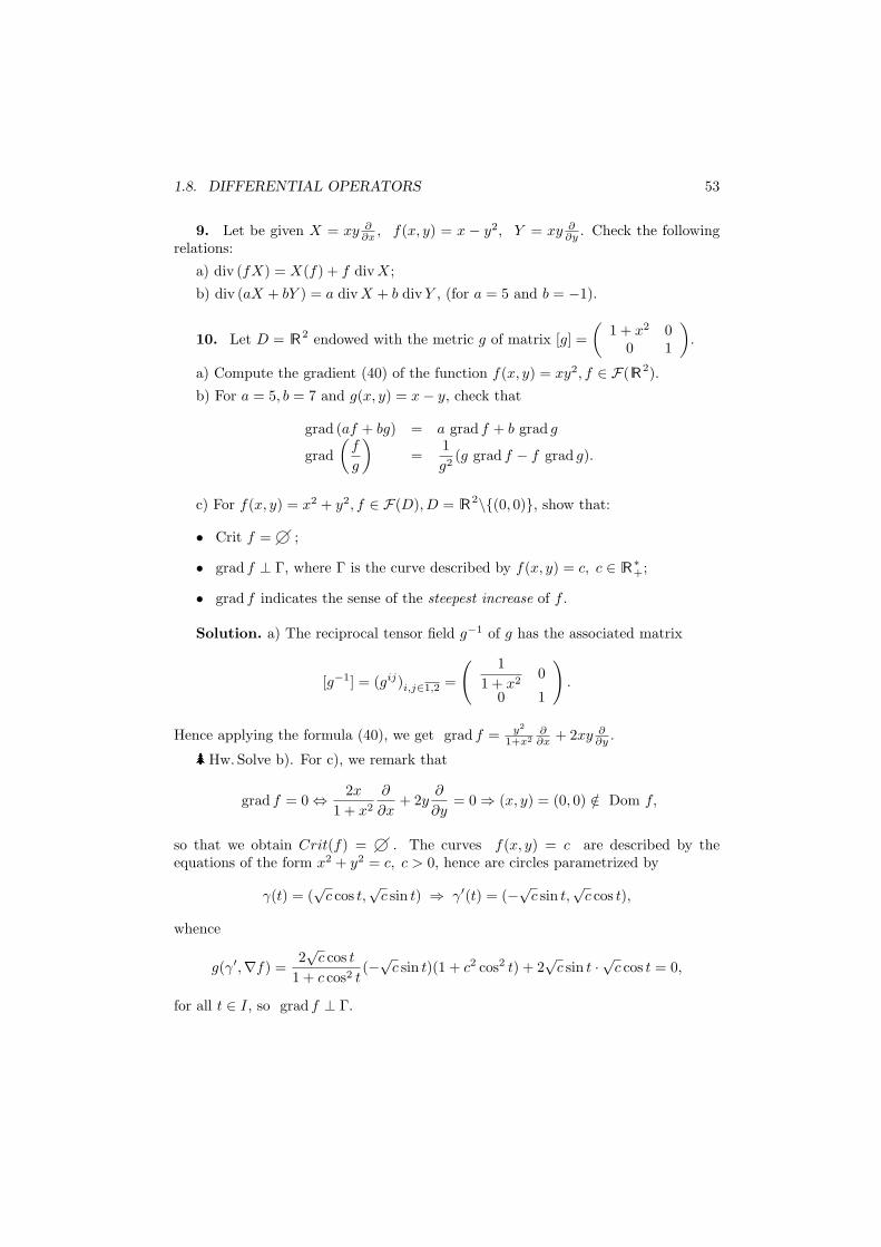
1.8. DIFFERENTIAL OPERATORS 53
9. Let be given X = xy ∂∂x , f(x, y) = x − y2, Y = xy ∂
∂y . Check the followingrelations:
a) div (fX) = X(f) + f divX;
b) div (aX + bY ) = a div X + b divY , (for a = 5 and b = −1).
10. Let D = R2 endowed with the metric g of matrix [g] =(
1 + x2 00 1
).
a) Compute the gradient (40) of the function f(x, y) = xy2, f ∈ F(R2).
b) For a = 5, b = 7 and g(x, y) = x− y, check that
grad (af + bg) = a grad f + b grad g
grad(
f
g
)=
1g2
(g grad f − f grad g).
c) For f(x, y) = x2 + y2, f ∈ F(D), D = R2\(0, 0), show that:
• Crit f = g¡ ;
• grad f ⊥ Γ, where Γ is the curve described by f(x, y) = c, c ∈ R∗+;
• grad f indicates the sense of the steepest increase of f .
Solution. a) The reciprocal tensor field g−1 of g has the associated matrix
[g−1] = (gij)i,j∈1,2 =
( 11 + x2
0
0 1
).
Hence applying the formula (40), we get grad f = y2
1+x2∂∂x + 2xy ∂
∂y .
Hw. Solve b). For c), we remark that
grad f = 0 ⇔ 2x
1 + x2
∂
∂x+ 2y
∂
∂y= 0 ⇒ (x, y) = (0, 0) /∈ Dom f,
so that we obtain Crit(f) = g¡ . The curves f(x, y) = c are described by theequations of the form x2 + y2 = c, c > 0, hence are circles parametrized by
γ(t) = (√
c cos t,√
c sin t) ⇒ γ′(t) = (−√c sin t,√
c cos t),
whence
g(γ′,∇f) =2√
c cos t
1 + c cos2 t(−√c sin t)(1 + c2 cos2 t) + 2
√c sin t · √c cos t = 0,
for all t ∈ I, so grad f ⊥ Γ.
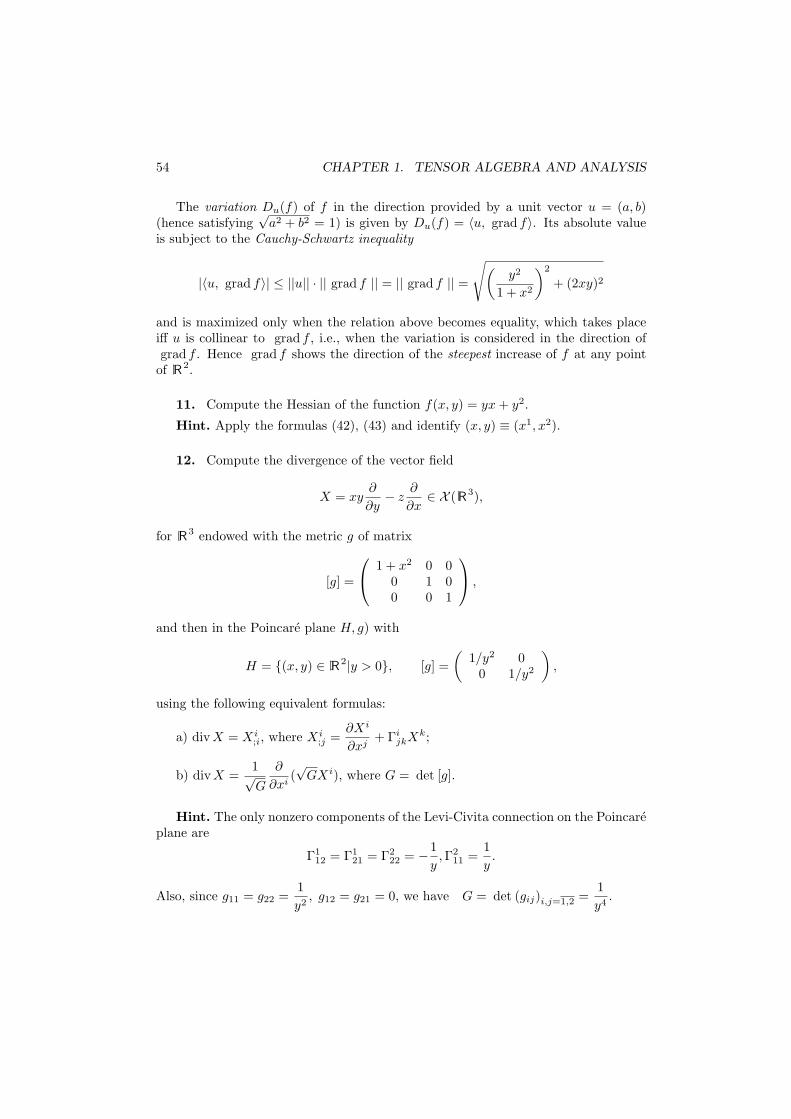
54 CHAPTER 1. TENSOR ALGEBRA AND ANALYSIS
The variation Du(f) of f in the direction provided by a unit vector u = (a, b)(hence satisfying
√a2 + b2 = 1) is given by Du(f) = 〈u, grad f〉. Its absolute value
is subject to the Cauchy-Schwartz inequality
|〈u, grad f〉| ≤ ||u|| · || grad f || = || grad f || =√(
y2
1 + x2
)2
+ (2xy)2
and is maximized only when the relation above becomes equality, which takes placeiff u is collinear to grad f , i.e., when the variation is considered in the direction ofgrad f . Hence grad f shows the direction of the steepest increase of f at any point
of R2.
11. Compute the Hessian of the function f(x, y) = yx + y2.
Hint. Apply the formulas (42), (43) and identify (x, y) ≡ (x1, x2).
12. Compute the divergence of the vector field
X = xy∂
∂y− z
∂
∂x∈ X (R3),
for R3 endowed with the metric g of matrix
[g] =
1 + x2 0 00 1 00 0 1
,
and then in the Poincare plane H, g) with
H = (x, y) ∈ R2|y > 0, [g] =(
1/y2 00 1/y2
),
using the following equivalent formulas:
a) div X = Xi;i, where Xi
;j =∂Xi
∂xj+ Γi
jkXk;
b) div X =1√G
∂
∂xi(√
GXi), where G = det [g].
Hint. The only nonzero components of the Levi-Civita connection on the Poincareplane are
Γ112 = Γ1
21 = Γ222 = −1
y, Γ2
11 =1y.
Also, since g11 = g22 =1y2
, g12 = g21 = 0, we have G = det (gij)i,j=1,2 =1y4
.
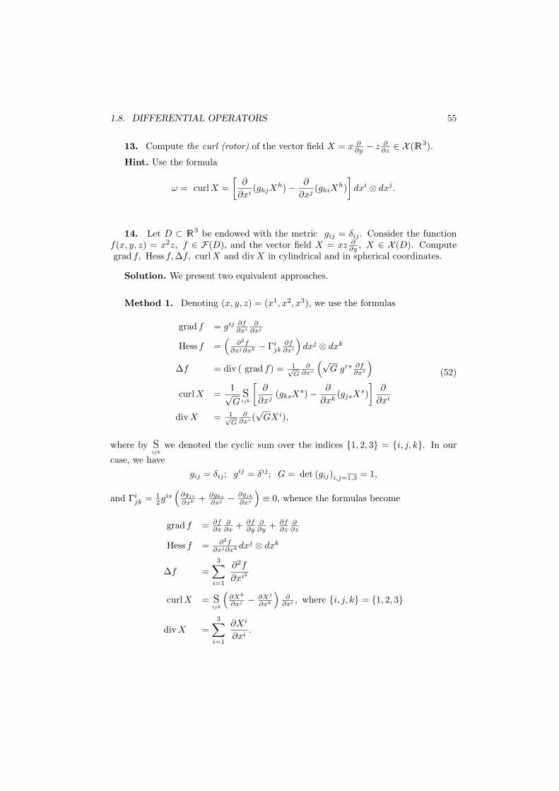
1.8. DIFFERENTIAL OPERATORS 55
13. Compute the curl (rotor) of the vector field X = x ∂∂y − z ∂
∂z ∈ X (R3).
Hint. Use the formula
ω = curl X =[
∂
∂xi(ghjX
h)− ∂
∂xj(ghiX
h)]
dxi ⊗ dxj .
14. Let D ⊂ R3 be endowed with the metric gij = δij . Consider the functionf(x, y, z) = x2z, f ∈ F(D), and the vector field X = xz ∂
∂y , X ∈ X (D). Computegrad f, Hess f, ∆f, curl X and div X in cylindrical and in spherical coordinates.
Solution. We present two equivalent approaches.
Method 1. Denoting (x, y, z) = (x1, x2, x3), we use the formulas
grad f = gij ∂f∂xi
∂∂xj
Hess f =(
∂2f∂xj∂xk − Γi
jk∂f∂xi
)dxj ⊗ dxk
∆f = div ( grad f) = 1√G
∂∂xs
(√G grs ∂f
∂xr
)
curlX =1√G
Sijk
[∂
∂xj(gksX
s)− ∂
∂xk(gjsX
s)]
∂
∂xi
divX = 1√G
∂∂xi (
√GXi),
(52)
where by Sijk
we denoted the cyclic sum over the indices 1, 2, 3 = i, j, k. In our
case, we havegij = δij ; gij = δij ; G = det (gij)i,j=1,3 = 1,
and Γijk = 1
2gis(
∂gjs
∂xk + ∂gks
∂xj − ∂gjk
∂xs
)≡ 0, whence the formulas become
grad f = ∂f∂x
∂∂x + ∂f
∂y∂∂y + ∂f
∂z∂∂z
Hess f = ∂2f∂xj∂xk dxj ⊗ dxk
∆f =3∑
i=1
∂2f
∂xi2
curlX = Sijk
(∂Xk
∂xj − ∂Xj
∂xk
)∂
∂xi , where i, j, k = 1, 2, 3
divX =3∑
i=1
∂Xi
∂xi.
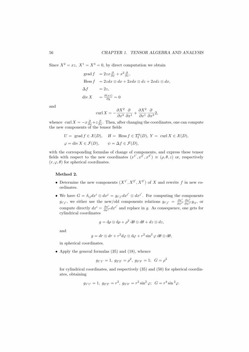
56 CHAPTER 1. TENSOR ALGEBRA AND ANALYSIS
Since X2 = xz, X1 = X3 = 0, by direct computation we obtain
grad f = 2zx ∂∂x + x2 ∂
∂z ,
Hess f = 2zdx⊗ dx + 2xdx⊗ dz + 2xdz ⊗ dx,
∆f = 2z,
divX = ∂(xz)∂y = 0
and
curlX = −∂X2
∂x3
∂
∂x1+
∂X2
∂x1
∂
∂x32,
whence curl X = −x ∂∂x +z ∂
∂z . Then, after changing the coordinates, one can computethe new components of the tensor fields
U = grad f ∈ X (D), H = Hess f ∈ T 02 (D), Y = curl X ∈ X (D),
ϕ = divX ∈ F(D), ψ = ∆f ∈ F(D),
with the corresponding formulas of change of components, and express these tensorfields with respect to the new coordinates (x1′ , x2′ , x3′) ≡ (ρ, θ, z) or, respectively(r, ϕ, θ) for spherical coordinates.
Method 2.
• Determine the new components (X1′ , X2′ , X3′) of X and rewrite f in new co-ordinates.
• We have G = δijdxi ⊗ dxj = gi′j′dxi′ ⊗ dxj′ . For computing the componentsgi′j′ , we either use the new/old components relations gi′j′ = ∂xi
∂xi′∂xj
∂xj′ gij , or
compute directly dxi = ∂xi
∂xi′ dxi′ and replace in g. As consequence, one gets forcylindrical coordinates
g = dρ⊗ dρ + ρ2 dθ ⊗ dθ + dz ⊗ dz,
andg = dr ⊗ dr + r2dϕ⊗ dϕ + r2 sin2 ϕ dθ ⊗ dθ,
in spherical coordinates.
• Apply the general formulas (35) and (18), whence
g1′1′ = 1, g2′2′ = ρ2, g3′3′ = 1; G = ρ2
for cylindrical coordinates, and respectively (35) and (50) for spherical coordin-ates, obtaining
g1′1′ = 1, g2′2′ = r2, g3′3′ = r2 sin2 ϕ; G = r4 sin 2ϕ.
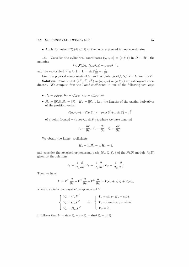
1.8. DIFFERENTIAL OPERATORS 57
• Apply formulas (47),(48),(49) to the fields expressed in new coordinates.
15. Consider the cylindrical coordinates (u, v, w) = (ρ, θ, z) in D ⊂ R3, themapping
f ∈ F(D), f(ρ, θ, z) = ρ cos θ + z,
and the vector field V ∈ X (D), V = sin θ ∂∂ρ − z ∂
∂θ .
Find the physical components of V , and compute grad f, ∆f, curl V and divV .
Solution. Remark that (x1′ , x2′ , x3′) = (u, v, w) = (ρ, θ, z) are orthogonal coor-dinates. We compute first the Lame coefficients in one of the following two ways
• Hu =√
g1′1′ , Hv =√
g2′2′ ,Hw =√
g3′3′ , or
• Hu = ||~ru||,Hv = ||~rv||,Hw = ||~rw||, i.e., the lengths of the partial derivativesof the position vector
~r(u, v, w) = ~r(ρ, θ, z) = ρ cos θ~i + ρ sin θ~j + z~k
of a point (x, y, z) = (ρ cos θ, ρ sin θ, z), where we have denoted
~ru =∂~r
∂u, ~rv =
∂~r
∂v, ~rw =
∂~r
∂w.
We obtain the Lame coefficients
Hu = 1,Hv = ρ,Hw = 1,
and consider the attached orthonormal basis ~eu, ~ev, ~ew of the F(D)-module X (D)given by the relations
~eu =1
Hu
∂
∂u, ~ev =
1Hv
∂
∂v, ~ew =
1Hw
∂
∂w.
Then we have
V = V 1′ ∂
∂u+ V 2′ ∂
∂v+ V 3′ ∂
∂w= Vu~eu + Vv~ev + Vw~ew,
whence we infer the physical components of V
Vu = HuX1′
Vv = HvX2′
Vw = HwX3′
⇒
Vu = sin v ·Hu = sin v
Vv = (−w) ·Hv = −wu
Vw = 0.
It follows that V = sin v ~eu − uw ~ev = sin θ ~eρ − ρz ~eθ.
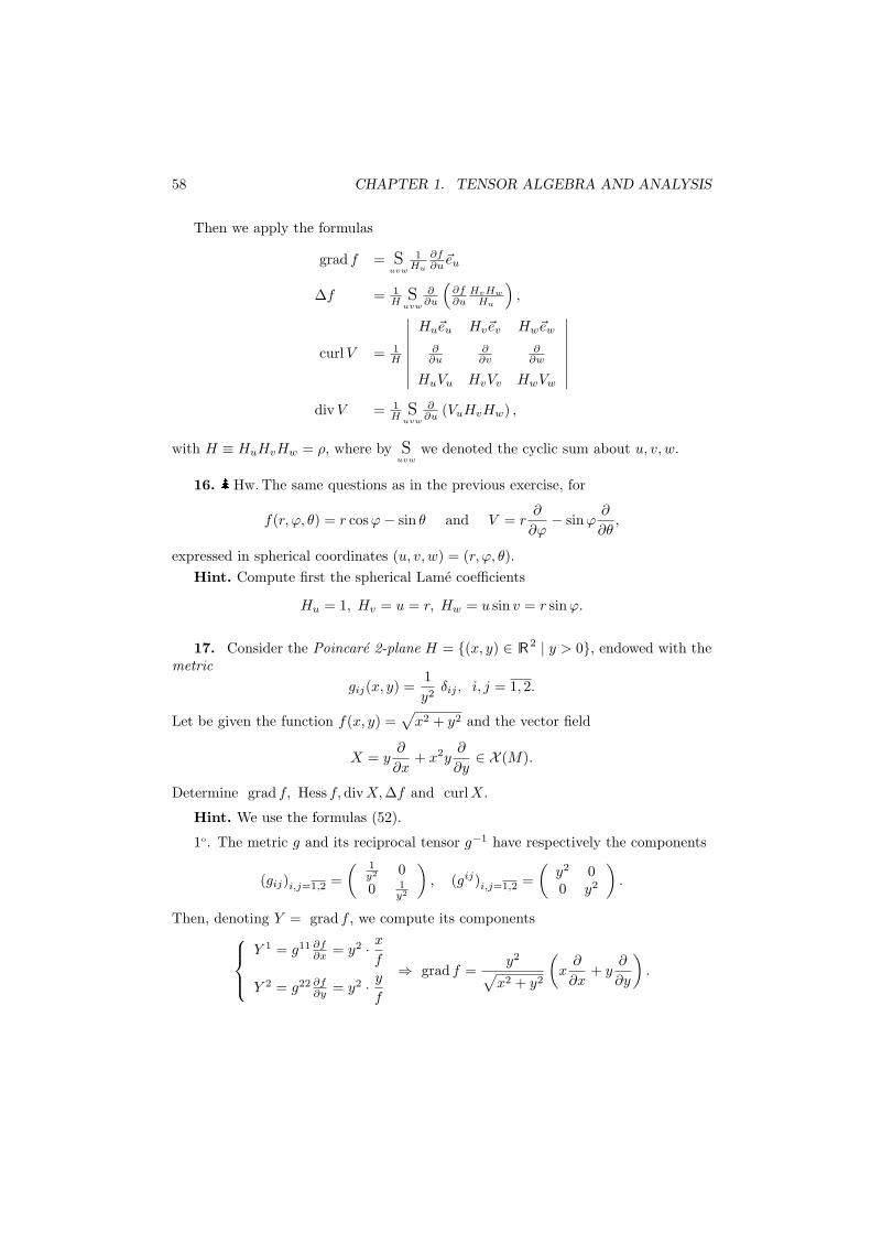
58 CHAPTER 1. TENSOR ALGEBRA AND ANALYSIS
Then we apply the formulas
grad f = Suvw
1Hu
∂f∂u~eu
∆f = 1H S
uvw
∂∂u
(∂f∂u
HvHw
Hu
),
curl V = 1H
∣∣∣∣∣∣∣∣
Hu~eu Hv~ev Hw~ew
∂∂u
∂∂v
∂∂w
HuVu HvVv HwVw
∣∣∣∣∣∣∣∣
div V = 1H S
uvw
∂∂u (VuHvHw) ,
with H ≡ HuHvHw = ρ, where by Suvw
we denoted the cyclic sum about u, v, w.
16. Hw.The same questions as in the previous exercise, for
f(r, ϕ, θ) = r cosϕ− sin θ and V = r∂
∂ϕ− sin ϕ
∂
∂θ,
expressed in spherical coordinates (u, v, w) = (r, ϕ, θ).Hint. Compute first the spherical Lame coefficients
Hu = 1, Hv = u = r, Hw = u sin v = r sin ϕ.
17. Consider the Poincare 2-plane H = (x, y) ∈ R2 | y > 0, endowed with themetric
gij(x, y) =1y2
δij , i, j = 1, 2.
Let be given the function f(x, y) =√
x2 + y2 and the vector field
X = y∂
∂x+ x2y
∂
∂y∈ X (M).
Determine grad f, Hess f, divX, ∆f and curl X.
Hint. We use the formulas (52).
1o. The metric g and its reciprocal tensor g−1 have respectively the components
(gij)i,j=1,2 =( 1
y2 00 1
y2
), (gij)i,j=1,2 =
(y2 00 y2
).
Then, denoting Y = grad f , we compute its components
Y 1 = g11 ∂f∂x = y2 · x
f
Y 2 = g22 ∂f∂y = y2 · y
f
⇒ grad f =y2
√x2 + y2
(x
∂
∂x+ y
∂
∂y
).
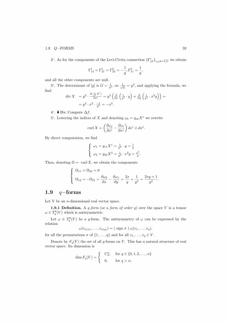
1.9. Q−FORMS 59
2o. As for the components of the Levi-Civita connection Γijki,j,k=1,3, we obtain
Γ112 = Γ1
21 = Γ222 = −1
y, Γ2
11 =1y,
and all the other components are null.3o. The determinant of [g] is G = 1
y4 , so 1√G
= y2, and applying the formula, wefind
div X = y2 · ∂( 1y2 Xi)
∂xi = y2(
∂∂x
(1y2 · y
)+ ∂
∂y
(1y2 · x2y
))=
= y2 · x2 · −1y2 = −x2.
4o. Hw. Compute ∆f .5o. Lowering the indices of X and denoting ωk = gskXs we rewrite
curl X =(
∂ωj
∂xi− ∂ωi
∂xj
)dxi ⊗ dxj .
By direct computation, we find
ω1 = g11X1 = 1
y2 · y = 1y
ω2 = g22X2 = 1
y2 · x2y = x2
y .
Then, denoting Ω = curl X, we obtain the components
Ω11 = Ω22 = 0
Ω12 = −Ω21 =∂ω2
∂x− ∂ω1
∂y=
2x
y+
1y2
=2xy + 1
y2.
1.9 q−forms
Let V be an n-dimensional real vector space.
1.9.1 Definition. A q-form (or a form of order q) over the space V is a tensorω ∈ T 0
q (V ) which is antisymmetric.
Let ω ∈ T 0q (V ) be a q-form. The antisymmetry of ω can be expressed by the
relationω(vσ(1), . . . , vσ(q)) = ( sign σ ) ω(v1, . . . , vq),
for all the permutations σ of 1, . . . , q and for all v1, . . . , vq ∈ V .
Denote by Fq(V ) the set of all q-forms on V . This has a natural structure of realvector space. Its dimension is
dim Fq(V ) =
Cq
n, for q ∈ 0, 1, 2, . . . , n0, for q > n.
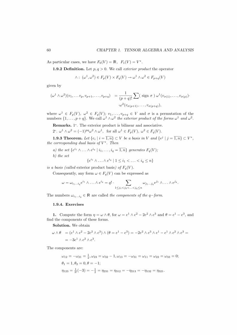
60 CHAPTER 1. TENSOR ALGEBRA AND ANALYSIS
As particular cases, we have F0(V ) = R , F1(V ) = V ∗.
1.9.2 Definition. Let p, q > 0. We call exterior product the operator
∧ : (ω1, ω2) ∈ Fp(V )× Fq(V ) → ω1 ∧ ω2 ∈ Fp+q(V )
given by
(ω1 ∧ ω2)(v1, . . . vp, vp+1, . . . , vp+q) =1
(p + q)!
∑( sign σ ) ω1(vσ(1), . . . , vσ(p))·
·ω2(vσ(p+1), . . . , vσ(p+q)),
where ω1 ∈ Fp(V ), ω2 ∈ Fq(V ); v1, . . . , vp+q ∈ V and σ is a permutation of thenumbers 1, . . . , p + q. We call ω1 ∧ ω2 the exterior product of the forms ω1 and ω2.
Remarks. 1o. The exterior product is bilinear and associative.2o. ω1 ∧ ω2 = (−1)pqω2 ∧ ω1, for all ω1 ∈ Fp(V ), ω2 ∈ Fq(V ).
1.9.3 Theorem. Let ei | i = 1, n ⊂ V be a basis in V and ej | j = 1, n ⊂ V ∗,the corresponding dual basis of V ∗. Then
a) the set ei1 ∧ . . . ∧ eiq | i1, . . . , iq = 1, n generates Fq(V );b) the set
ei1 ∧ . . . ∧ eiq | 1 ≤ i1 < . . . < iq ≤ nis a basis (called exterior product basis) of Fq(V ).
Consequently, any form ω ∈ Fq(V ) can be expressed as
ω = ωi1...iqei1 ∧ . . . ∧ eiq = q! ·
∑
1≤j1<j2<...<jq≤n
ωj1...jqej1 ∧ . . . ∧ ejq .
The numbers ωi1...iq ∈ R are called the components of the q−form.
1.9.4. Exercises
1. Compute the form η = ω ∧ θ, for ω = e1 ∧ e2 − 2e2 ∧ e3 and θ = e1 − e3, andfind the components of these forms.
Solution. We obtain
ω ∧ θ = (e1 ∧ e2 − 2e2 ∧ e3) ∧ (θ = e1 − e3) = −2e2 ∧ e3 ∧ e1 − e1 ∧ e2 ∧ e3 =
= −3e1 ∧ e2 ∧ e3.
The components are:
ω12 = −ω21 = 12 , ω23 = ω32 − 1, ω13 = −ω31 = ω11 = ω22 = ω33 = 0;
θ1 = 1, θ2 = 0, θ = −1;
η123 = 13! (−3) = − 1
2 = η231 = η312 = −η213 = −η132 = η321.
1.10. DIFFERENTIAL Q−FORMS 61
2. Is ω = 4e1 ∧ e2 ∧ e3 a basis in F3(R3) ? But in F3(R4) ?
Solution. The 3-form ω is a basis in the vector space F3( R3), since it is linearlyindependent (being nonzero form) and dim F3(R3) = 1.
On the other hand, ω is not a basis of F3(R4), since it generates just an 1-dimensional vector subspace of the C3
4=4-dimensional vector space F3(R4). However,it can be completed to a basis of F3(R4), e.g.,
ω, e1 ∧ e3 ∧ e4, e2 ∧ e3 ∧ e4, e1 ∧ e2 ∧ e4.
1.10 Differential q−forms
Let us consider the path integral∫
γ
[P (x, y, z)dx + Q(x, y, z)dy + R(x, y, z)dz]
and the surface integral∫
σ
[P (x, y, z)dy ∧ dz + Q(x, y, z)dz ∧ dx + R(x, y, z)dx ∧ dy] .
If P, Q, R are differentiable functions, then the mathematical object
P (x, y, z)dx + Q(x, y, z)dy + R(x, y, z)dz
is called differential 1-form, and the object
P (x, y, z) dy ∧ dz + Q(x, y, z) dz ∧ dx + R(x, y, z) dx ∧ dy
is called differential 2-form.We introduce the general notion of differential q-form as follows. Let D ⊂ Rn be
an open subset of Rn, let x = (x1, . . . , xn) ∈ D, V = TxD, and let Fq(TxD) be theset of all q-forms on TxD.
1.10.1 Definition. A differentiable function ω : D → ⋃x∈D
Fq(TxD) such that
ω(x) ∈ Fq(TxD), for all x ∈ D,
is called differential q−form (or a field of q-forms).Let Fq(D) be the set of all differential q-forms on D. It has a canonical struc-
ture of real vector space and of an F(D)−module. Regarding the last structure, ifB =
∂
∂xi , i = 1, n
is a basis in X (D) and B∗ =dxi, i = 1, n
⊂ X ∗(D) is thecorresponding dual basis, then the induced set of generators is
dxi1 ∧ . . . ∧ dxiq | i1, . . . , iq ∈ 1, n,
62 CHAPTER 1. TENSOR ALGEBRA AND ANALYSIS
and the induced basis in Fq(D) isdxi1 ∧ . . . ∧ dxiq | 1 ≤ i1 < i2 < . . . < iq ≤ n
⊂ Fq(D).
Consequently, any differential form ω ∈ Fq(D) decomposes like
ω = ωi1...iqdxi1 ∧ . . . ∧ dxiq =
= q!∑
1≤j1<...<jq≤n
ωj1...jqej1 ∧ . . . ∧ ejq ,
where ωi1,...,iq∈ F(D) are called the components of the differential q−form.
1.10.2 Operations with forms
1.10.2.1 Definition. The interior product is the application
: X (D)×Fq(D) → Fq−1(D),
given by(X ω)(X1, . . . , Xq−1) = ω(X, X1, . . . , Xq−1),
for all Xi ∈ X (D), i = 1, q − 1. Then the differential (p − 1)−form X ω ∈ Fq−1(D)is called also the interior product between X and ω.
The components of X ω are given by
(X ω)i2...iq = Xi1ωi1i2...iq , i2, . . . , iq = 1, n.
Consequently, X ω is the tensor product X ⊗ ω followed by a suitable transvection.
1.10.2.2 Definition. The function d : Fq(D) → Fq+1(D), for all q ≥ 0, whichsatisfies
a) d2 = 0;b) d(ω1 ∧ ω2) = dω1 ∧ ω2 + (−1)pqω1 ∧ dω2, for all ω1 ∈ Fp(D), ω2 ∈ Fq(D);c) X(dω) = d(X(ω)), where
X(ω) = X dω + d(X ω), for all X ∈ X (D), ω ∈ Fp(D);
d) d(f) = df, for all f ∈ F0(D) ≡ F(D),
is called exterior differentiation.
Generally, for a differential q−form ω = ωi1...ipdxi1 ∧ . . . ∧ dxiq , we have
dω = dωi1...iq ∧ dxi1 ∧ . . . ∧ dxiq .
In particular:
1.10. DIFFERENTIAL Q−FORMS 63
• for ω = ωidxi ∈ F1(D), D ⊂ R3, we obtain
dω = dωi ∧ dxi =∂ωi
∂xjdxj ∧ dxi =
(∂ω3
∂x2− ∂ω2
∂x3
)dx2 ∧ dx3+
+(
∂ω1
∂x3− ∂ω3
∂x1
)dx3 ∧ dx1 +
(∂ω2
∂x1− ∂ω1
∂x2
)dx1 ∧ dx2,
• for η = ηijdxi ∧ dxj ∈ F2(D), D ⊂ R3, we obtain
dη = ∂ηij
∂xk dxi ∧ dxj ∧ dxk =
= 2(
∂η12∂x3 + ∂η31
∂x2 + ∂η23∂x1
)dx1 ∧ dx2 ∧ dx3,
where we used the relations
dωi =∂ωi
∂xjdxj , dxi ∧ dxi = 0, dxi ∧ dxj = −dxj ∧ dxi, for all i, j = 1, n.
1.10.2.3 Definitions. a) A differential form ω ∈ Fq(D) is called closed iff dω = 0.b) If there exist η ∈ Fq−1(D) such that ω = dη, then ω is called an exact form.
1.10.2.4 Remarks. For D ⊂ R3 endowed with the metric g = δijdxi ⊗ dxj , the1-forms and the 2-forms can be converted into vector fields using the rules
ω = ωi dxi ∈ F1(D) ↔(1)
3∑
i=1
ωi∂
∂xi∈ X (D)
ω = ωi dxi ∈ F1(D) ↔(2)
ω1 dx2 ∧ dx3 + ω2 dx3 ∧ dx1 + ω3 dx1 ∧ dx2 ∈ F2(D).
The correspondence df ∈ F1(D) ↔(1)
grad f ∈ X (D), can be extended to
ω = ωi dxi↔(1)
X = Xi ∂
∂xi∈ X (D), ω ∈ F1(D)
by means of the relationsωi = δisX
s; Xi = δisωs. (53)
Particularly, we have the correspondence
η = dω ∈ F2(D) ↔(2)
Y = curl X ∈ X (D),
which is given in general by
η =∑
i<j
ηijdxi ∧ dxj ∈ F2(D) ↔(2)
Y i ∂
∂xi∈ X (D),
64 CHAPTER 1. TENSOR ALGEBRA AND ANALYSIS
with η12 = Y 3, η23 = Y 1, η31 = Y 2.
Also the correspondence η↔(2)
Y yields the relation
dη = (div Y ) dx1 ∧ dx2 ∧ dx3.
1.10.3. Exercises
1. Let X = x ∂∂z ∈ X (D), D ⊂ R3 and
ω = xzdx ∧ dy − ydy ∧ dz.
Compute the following tensor fields:
a) X ω, where X = x∂
∂z, ω = xz dx ∧ dy − y dy ∧ dz;
b) dω, where ω = xz dx ∧ dy − y dy ∧ dz;
c) ω ∧ η, η ∧ ω, where η = xdx + 2ydz;
d) df, d2f , where f(x, y, z) = x + 2yz.
Consider as well the case ω = xdy + ydz.
Solution. a) If X = Xi ∂∂xi and ω = ωi1...ipdxi1 ∧ . . . ∧ dxip , then
(X ω) = Xi1ωi1i2...ipdxi2 ∧ . . . ∧ dxip .
For ω = xzdx∧ dy− ydy∧ dz ∈ F2(D) and X = x ∂∂z ∈ X (D), denoting (x1, x2, x3) ≡
(x, y, z) and identifying then with the decompositions
ω = ωijdxi ∧ dxj , X = Xi ∂
∂xi,
we obtain the components
ω12 = xz = −ω21, ω23 = −y = −ω32, ω31 = ω13 = 0 ⇒ [ω] =
0 xz 0−xz 0 −y
0 y 0
and respectively X1 = X2 = 0, X3 = x. Then, for θ = (X ω) = θidxi ∈ F1(D),with θi = Xkωki, i = 1, 3, we obtain
θ1 = X1ω11 + X2ω21 + X3ω31 = 0
θ2 = X1ω12 + X2ω22 + X3ω32 = xy
θ3 = X1ω13 + X2ω23 + X3ω33 = 0
⇒ X ω = xydy.
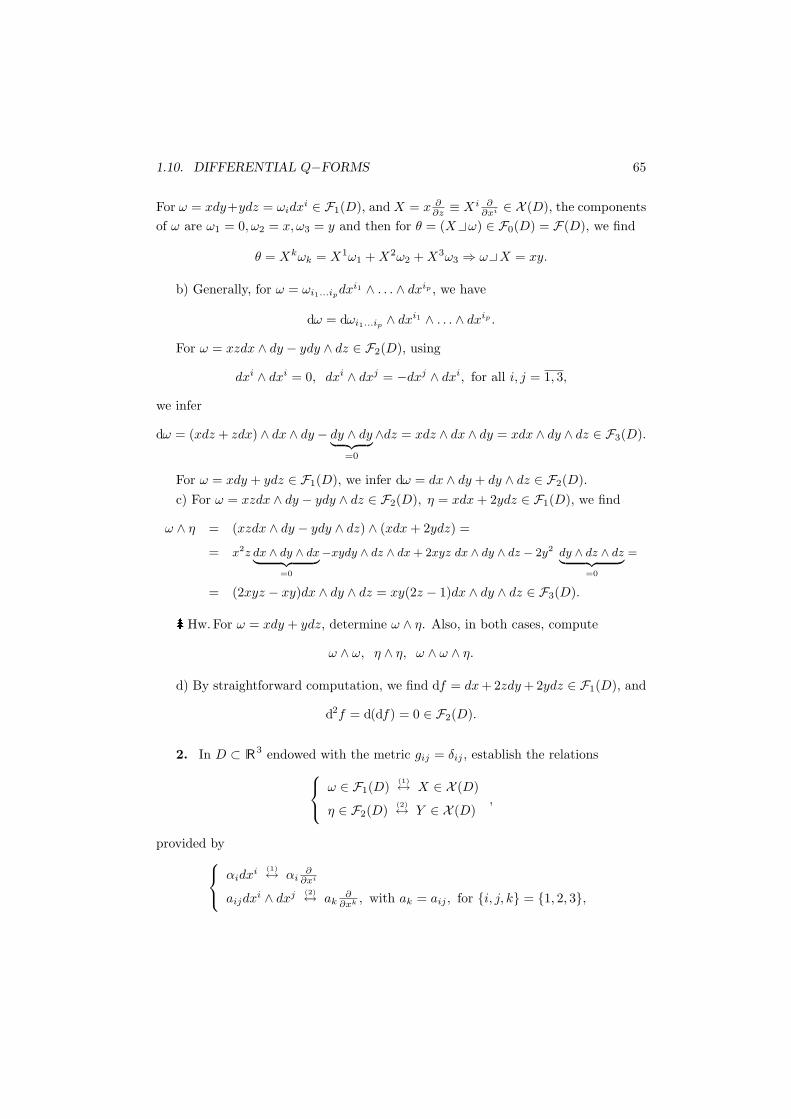
1.10. DIFFERENTIAL Q−FORMS 65
For ω = xdy+ydz = ωidxi ∈ F1(D), and X = x ∂∂z ≡ Xi ∂
∂xi ∈ X (D), the componentsof ω are ω1 = 0, ω2 = x, ω3 = y and then for θ = (X ω) ∈ F0(D) = F(D), we find
θ = Xkωk = X1ω1 + X2ω2 + X3ω3 ⇒ ω X = xy.
b) Generally, for ω = ωi1...ipdxi1 ∧ . . . ∧ dxip , we have
dω = dωi1...ip∧ dxi1 ∧ . . . ∧ dxip .
For ω = xzdx ∧ dy − ydy ∧ dz ∈ F2(D), using
dxi ∧ dxi = 0, dxi ∧ dxj = −dxj ∧ dxi, for all i, j = 1, 3,
we infer
dω = (xdz + zdx) ∧ dx ∧ dy − dy ∧ dy︸ ︷︷ ︸=0
∧dz = xdz ∧ dx ∧ dy = xdx ∧ dy ∧ dz ∈ F3(D).
For ω = xdy + ydz ∈ F1(D), we infer dω = dx ∧ dy + dy ∧ dz ∈ F2(D).c) For ω = xzdx ∧ dy − ydy ∧ dz ∈ F2(D), η = xdx + 2ydz ∈ F1(D), we find
ω ∧ η = (xzdx ∧ dy − ydy ∧ dz) ∧ (xdx + 2ydz) =
= x2z dx ∧ dy ∧ dx︸ ︷︷ ︸=0
−xydy ∧ dz ∧ dx + 2xyz dx ∧ dy ∧ dz − 2y2 dy ∧ dz ∧ dz︸ ︷︷ ︸=0
=
= (2xyz − xy)dx ∧ dy ∧ dz = xy(2z − 1)dx ∧ dy ∧ dz ∈ F3(D).
Hw.For ω = xdy + ydz, determine ω ∧ η. Also, in both cases, compute
ω ∧ ω, η ∧ η, ω ∧ ω ∧ η.
d) By straightforward computation, we find df = dx + 2zdy + 2ydz ∈ F1(D), and
d2f = d(df) = 0 ∈ F2(D).
2. In D ⊂ R3 endowed with the metric gij = δij , establish the relations
ω ∈ F1(D) (1)↔ X ∈ X (D)
η ∈ F2(D) (2)↔ Y ∈ X (D),
provided by
αidxi (1)↔ αi∂
∂xi
aijdxi ∧ dxj (2)↔ ak∂
∂xk , with ak = aij , for i, j, k = 1, 2, 3,
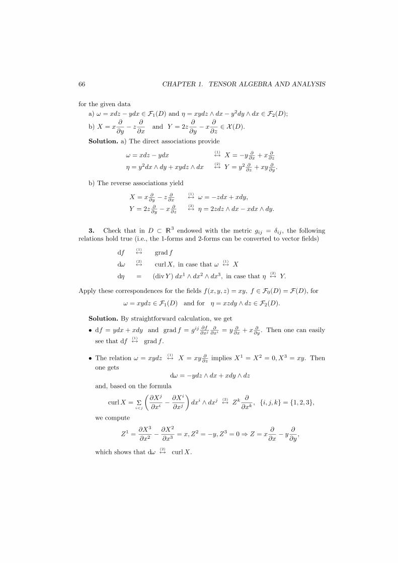
66 CHAPTER 1. TENSOR ALGEBRA AND ANALYSIS
for the given dataa) ω = xdz − ydx ∈ F1(D) and η = xydz ∧ dx− y2dy ∧ dx ∈ F2(D);
b) X = x∂
∂y− z
∂
∂xand Y = 2z
∂
∂y− x
∂
∂z∈ X (D).
Solution. a) The direct associations provide
ω = xdz − ydx(1)↔ X = −y ∂
∂x + x ∂∂z
η = y2dx ∧ dy + xydz ∧ dx(2)↔ Y = y2 ∂
∂z + xy ∂∂y .
b) The reverse associations yield
X = x ∂∂y − z ∂
∂x
(1)↔ ω = −zdx + xdy,
Y = 2z ∂∂y − x ∂
∂z
(2)↔ η = 2zdz ∧ dx− xdx ∧ dy.
3. Check that in D ⊂ R3 endowed with the metric gij = δij , the followingrelations hold true (i.e., the 1-forms and 2-forms can be converted to vector fields)
df(1)↔ grad f
dω(2)↔ curl X, in case that ω
(1)↔ X
dη = (div Y ) dx1 ∧ dx2 ∧ dx3, in case that η(2)↔ Y.
Apply these correspondences for the fields f(x, y, z) = xy, f ∈ F0(D) = F(D), for
ω = xydz ∈ F1(D) and for η = xzdy ∧ dz ∈ F2(D).
Solution. By straightforward calculation, we get
• df = ydx + xdy and grad f = gij ∂f∂xj
∂∂xi = y ∂
∂x + x ∂∂y . Then one can easily
see that df(1)↔ grad f .
• The relation ω = xydz(1)↔ X = xy ∂
∂z implies X1 = X2 = 0, X3 = xy. Thenone gets
dω = −ydz ∧ dx + xdy ∧ dz
and, based on the formula
curl X = Σi<j
(∂Xj
∂xi− ∂Xi
∂xj
)dxi ∧ dxj (2)↔ Zk ∂
∂xk, i, j, k = 1, 2, 3,
we compute
Z1 =∂X3
∂x2− ∂X2
∂x3= x,Z2 = −y, Z3 = 0 ⇒ Z = x
∂
∂x− y
∂
∂y,
which shows that dω(2)↔ curl X.
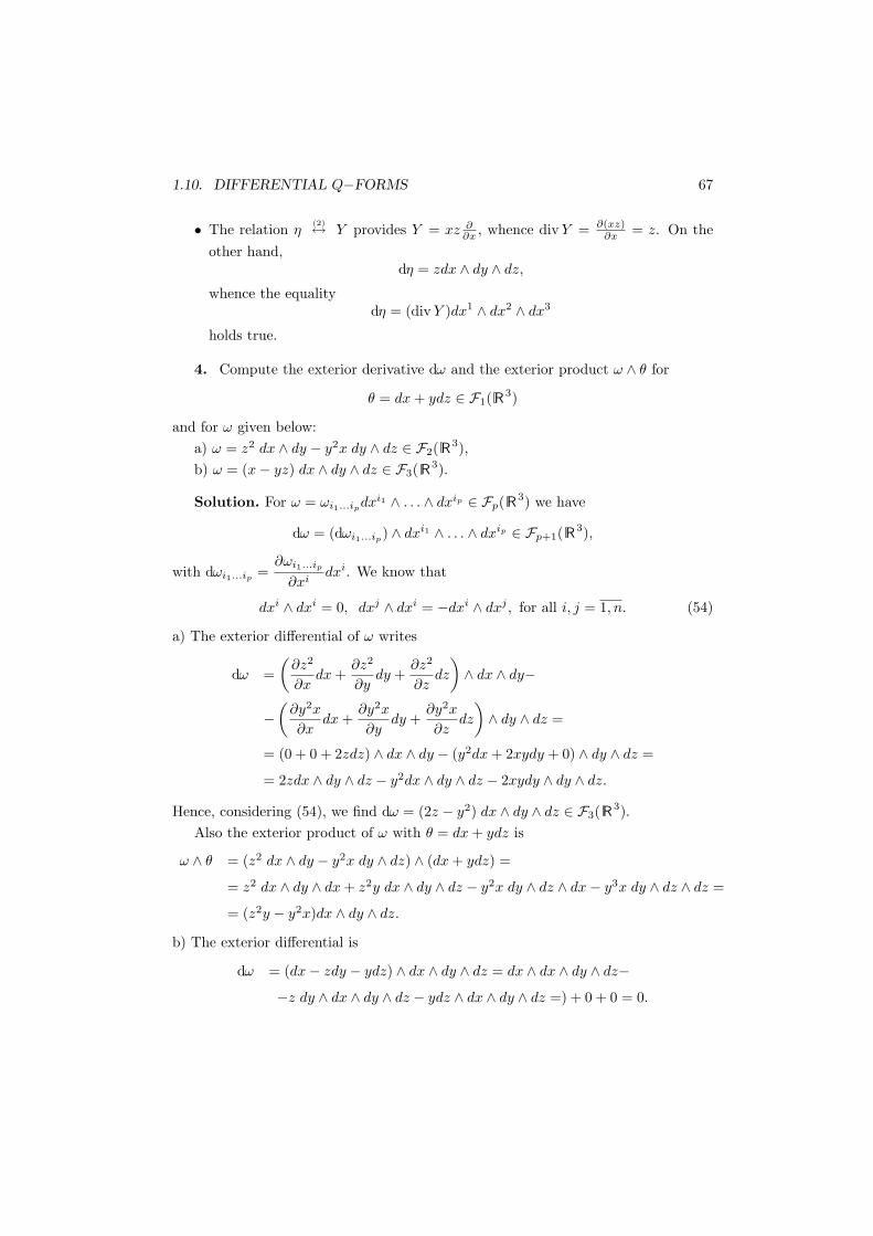
1.10. DIFFERENTIAL Q−FORMS 67
• The relation η(2)↔ Y provides Y = xz ∂
∂x , whence div Y = ∂(xz)∂x = z. On the
other hand,dη = zdx ∧ dy ∧ dz,
whence the equalitydη = (div Y )dx1 ∧ dx2 ∧ dx3
holds true.
4. Compute the exterior derivative dω and the exterior product ω ∧ θ for
θ = dx + ydz ∈ F1(R3)
and for ω given below:a) ω = z2 dx ∧ dy − y2x dy ∧ dz ∈ F2(R3),b) ω = (x− yz) dx ∧ dy ∧ dz ∈ F3(R3).
Solution. For ω = ωi1...ipdxi1 ∧ . . . ∧ dxip ∈ Fp(R3) we have
dω = (dωi1...ip) ∧ dxi1 ∧ . . . ∧ dxip ∈ Fp+1( R3),
with dωi1...ip =∂ωi1...ip
∂xidxi. We know that
dxi ∧ dxi = 0, dxj ∧ dxi = −dxi ∧ dxj , for all i, j = 1, n. (54)
a) The exterior differential of ω writes
dω =(
∂z2
∂xdx +
∂z2
∂ydy +
∂z2
∂zdz
)∧ dx ∧ dy−
−(
∂y2x
∂xdx +
∂y2x
∂ydy +
∂y2x
∂zdz
)∧ dy ∧ dz =
= (0 + 0 + 2zdz) ∧ dx ∧ dy − (y2dx + 2xydy + 0) ∧ dy ∧ dz =
= 2zdx ∧ dy ∧ dz − y2dx ∧ dy ∧ dz − 2xydy ∧ dy ∧ dz.
Hence, considering (54), we find dω = (2z − y2) dx ∧ dy ∧ dz ∈ F3( R3).Also the exterior product of ω with θ = dx + ydz is
ω ∧ θ = (z2 dx ∧ dy − y2x dy ∧ dz) ∧ (dx + ydz) =
= z2 dx ∧ dy ∧ dx + z2y dx ∧ dy ∧ dz − y2x dy ∧ dz ∧ dx− y3x dy ∧ dz ∧ dz =
= (z2y − y2x)dx ∧ dy ∧ dz.
b) The exterior differential is
dω = (dx− zdy − ydz) ∧ dx ∧ dy ∧ dz = dx ∧ dx ∧ dy ∧ dz−−z dy ∧ dx ∧ dy ∧ dz − ydz ∧ dx ∧ dy ∧ dz =) + 0 + 0 = 0.
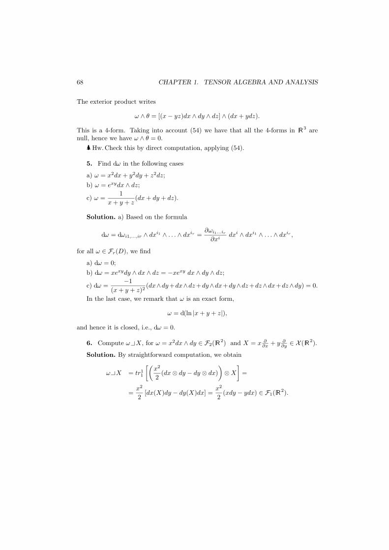
68 CHAPTER 1. TENSOR ALGEBRA AND ANALYSIS
The exterior product writes
ω ∧ θ = [(x− yz)dx ∧ dy ∧ dz] ∧ (dx + ydz).
This is a 4-form. Taking into account (54) we have that all the 4-forms in R3 arenull, hence we have ω ∧ θ = 0.
Hw.Check this by direct computation, applying (54).
5. Find dω in the following cases
a) ω = x2dx + y2dy + z2dz;b) ω = exydx ∧ dz;
c) ω =1
x + y + z(dx + dy + dz).
Solution. a) Based on the formula
dω = dωi1,...,ir ∧ dxi1 ∧ . . . ∧ dxir =∂ωi1...ir
∂xidxi ∧ dxi1 ∧ . . . ∧ dxir ,
for all ω ∈ Fr(D), we find
a) dω = 0;b) dω = xexydy ∧ dx ∧ dz = −xexy dx ∧ dy ∧ dz;
c) dω =−1
(x + y + z)2(dx∧dy +dx∧dz +dy∧dx+dy∧dz +dz∧dx+dz∧dy) = 0.
In the last case, we remark that ω is an exact form,
ω = d(ln |x + y + z|),
and hence it is closed, i.e., dω = 0.
6. Compute ω X, for ω = x2dx ∧ dy ∈ F2(R2) and X = x ∂∂x + y ∂
∂y ∈ X ( R2).
Solution. By straightforward computation, we obtain
ω X = tr11
[(x2
2(dx⊗ dy − dy ⊗ dx)
)⊗X
]=
=x2
2[dx(X)dy − dy(X)dx] =
x2
2(xdy − ydx) ∈ F1( R2).
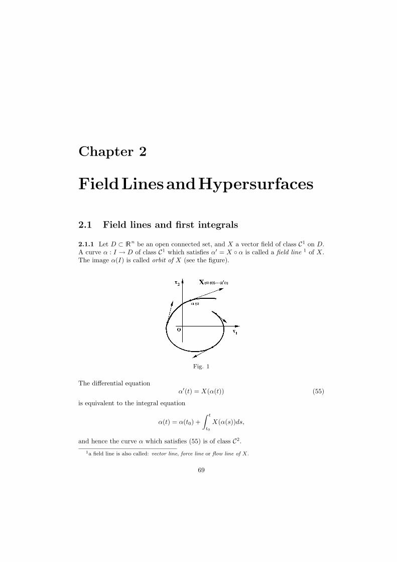
Chapter 2
FieldLinesandHypersurfaces
2.1 Field lines and first integrals
2.1.1 Let D ⊂ Rn be an open connected set, and X a vector field of class C1 on D.A curve α : I → D of class C1 which satisfies α′ = X α is called a field line 1 of X.The image α(I) is called orbit of X (see the figure).
Fig. 1
The differential equationα′(t) = X(α(t)) (55)
is equivalent to the integral equation
α(t) = α(t0) +∫ t
t0
X(α(s))ds,
and hence the curve α which satisfies (55) is of class C2.
1a field line is also called: vector line, force line or flow line of X.
69
70 CHAPTER 2. FIELD LINES AND HYPERSURFACES
Explicitly, for X = (X1, . . . , Xn) and
α = (x1, . . . , xn), x1 = x1(t), . . . , xn = xn(t), t ∈ I,
the vector differential equation (55) is written under the form of an autonomousdifferential system
dx1
dt= X1(x1, . . . , xn)
. . .
dxn
dt= Xn(x1, . . . , xn).
(56)
The existence and uniqueness theorem for a Cauchy problem associated to thissystem can be reformulated as
2.1.2 Theorem. If X is a vector field of class C1, then for any x0 ∈ D, t0 ∈ R ,there exists an open interval I and a field line α : I → D with the properties:
a) α(t0) = x0;b) if β : J → D is any other field line of X such that β(t1) = x0, then J ⊆ I and
β(t) = α(t− t0 + t1), for all t ∈ J.
The curve α is called the maximal field line of X which passes through x0.
Definition. The solutions a ∈ D of the algebraic autonomous system
X1(x1, . . . , xn) = 0, . . . , Xn(x1, . . . , xn) = 0, (57)
are called zeros of X. The constant solutions x(t) = a, t ∈ R of the differentialsystem (56) are called equilibrium points of X.
Example. Find the field lines and the equilibrium points of the field
X(x1, x2) = (−x2, x1).
Solution. By integration, one obtains the general solution
x1(t) = C1 cos t + C2 sin tx2(t) = C1 sin t− C2 cos t,
which for the initial conditions x1(0) = ax2(0) = b
provides the particular solution which passes through the point (a, b) at the momentt0 = 0, given by
x1(t) = a cos t− b sin tx2(t) = a sin t + b cos t.
2.1. FIELD LINES AND FIRST INTEGRALS 71
The unique equilibrium point of X is the origin O(0, 0).
Properties of field lines.
1) The reparametrizations by translations are admitted.2) Two distinct maximal field lines of X have in common no point.3) Any maximal field line is either injective, either simple and closed, or constant.
Assume that ϕ : D → D∗, y = ϕ(x) is a diffeomorphism of class C1. The system
dxi
dt= Xi(x)
is equivalent todyj
dt=
n∑
i=1
(∂yj
∂xiXi
)(ϕ−1(y)), j = 1, n,
or, equivalently,dyj
dt= (DXyj)(ϕ−1(y)).
The following theorem gives conditions under which DXyj =
0, for j = 1, n− 11, for j = n.
2.1.3 Theorem (Rectification Theorem). If X = (X1, . . . , Xn) is a vectorfield of class C1 on D and x0 satisfies X(x0) 6= 0, then there exists a neighborhood Uof x0 and a diffeomorphism ϕ : U → V ⊂ Rn, y = ϕ(x) of class C1, such that the
systemdxi
dt= Xi(x) on Ux0 is reduced to
dy1
dt= 0, . . . ,
dyn−1
dt= 0,
dyn
dt= 1
on the domain V = ϕ(U).Definition. A function f : D → R is called first integral for the differential
system (56) iff DXf = 0.This definition is equivalent to any of the two following assertions:
a) f is constant along any field line of X;b) any orbit of X is contained in one single set of constant level of f .
Hw.Check that the Hamiltonian function H : R2n → R is a (global) firstintegral of the Hamiltonian system
dxi
dt= −∂H
∂yi;
dyi
dt=
∂H
∂xi,
i.e., it satisfies DXH = 0, where X is the associated Hamiltonian field
X = (X1, . . . , Xn, Xn+1, . . . , X2n), Xi = −∂H
∂yi, Xn+i =
∂H
∂xi, i = 1, n.
72 CHAPTER 2. FIELD LINES AND HYPERSURFACES
2.1.4 Theorem. Let X be a field of class C1 on D, and x0 ∈ D, such that X(x0) 6=0. Then there exists a neighborhood Ux0 of x0 and n−1 first integrals f1, f2, . . . , fn−1,which are functional independent on Ux0 and any other first integral is a function ofclass C1 of f1, f2, . . . , fn−1. The orbits of X are described by the system of Cartesianequations f1(x) = C1, . . . , fn−1(x) = Cn−1, where C1, . . . , Cn−1 ∈ R .
Proof. By Theorem 1.3, there exists a diffeomorphism
y1 = f1(x), . . . , yn−1 = fn−1(x), yn = fn(x), x ∈ U,
such that DXfα = 0, α = 1, n− 1 and hence fα are first integrals.Let f1, . . . , fn−1 be first integrals; if f is another first integral, then DXfα = 0
and DXf = 0. Hence D(f,f1,...,fn−1)D(x1,...,xn) = 0, whence the functions f, f1, . . . , fn−1 are
functionally dependent, i.e., f = φ(f1, . . . , fn−1). 2
We note that the differential system of n equations (56) rewrites
dt =dx1
X1(x1, . . . , xn)= . . . =
dxn
Xn(x1, . . . , xn),
or, omitting dt, as
dx1
X1(x1, . . . , xn)= . . . =
dxn
Xn(x1, . . . , xn), (58)
which is called the symmetric differential system associated to the vector field X. Thenthe first integrals of X can be determined from (58) using the method of integrablecombinations: if there exist the functions λj : D → R , j ∈ 1, n and f : D → R suchthat
dx1
X1= . . . =
dxn
Xn=
n∑
j=1
λj(x)dxj
n∑
j=1
λjXj
=df
0, (59)
then it follows that df = 0, whence f is constant along the orbits of X, hence f is afirst integral for X. In this case, the differential
df =n∑
j=1
λj(x)dxj
which satisfies the conditionn∑
i=1
λi(x)Xi(x) = 0,
is called integrable combination of the symmetric system (58).
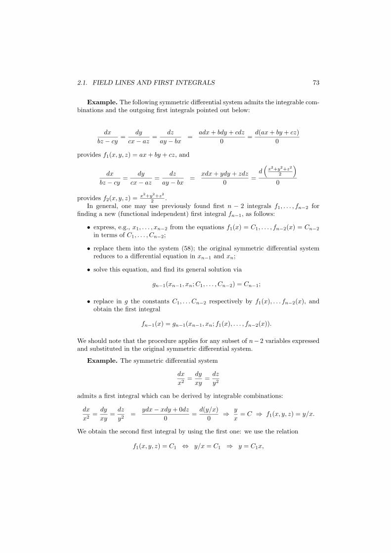
2.1. FIELD LINES AND FIRST INTEGRALS 73
Example. The following symmetric differential system admits the integrable com-binations and the outgoing first integrals pointed out below:
dx
bz − cy=
dy
cx− az=
dz
ay − bx=
adx + bdy + cdz
0=
d(ax + by + cz)0
provides f1(x, y, z) = ax + by + cz, and
dx
bz − cy=
dy
cx− az=
dz
ay − bx=
xdx + ydy + zdz
0=
d(
x2+y2+z2
2
)
0
provides f2(x, y, z) = x2+y2+z2
2 .In general, one may use previously found first n − 2 integrals f1, . . . , fn−2 for
finding a new (functional independent) first integral fn−1, as follows:
• express, e.g., x1, . . . , xn−2 from the equations f1(x) = C1, . . . , fn−2(x) = Cn−2
in terms of C1, . . . , Cn−2;
• replace them into the system (58); the original symmetric differential systemreduces to a differential equation in xn−1 and xn;
• solve this equation, and find its general solution via
gn−1(xn−1, xn; C1, . . . , Cn−2) = Cn−1;
• replace in g the constants C1, . . . Cn−2 respectively by f1(x), . . . fn−2(x), andobtain the first integral
fn−1(x) = gn−1(xn−1, xn; f1(x), . . . , fn−2(x)).
We should note that the procedure applies for any subset of n− 2 variables expressedand substituted in the original symmetric differential system.
Example. The symmetric differential system
dx
x2=
dy
xy=
dz
y2
admits a first integral which can be derived by integrable combinations:
dx
x2=
dy
xy=
dz
y2=
ydx− xdy + 0dz
0=
d(y/x)0
⇒ y
x= C ⇒ f1(x, y, z) = y/x.
We obtain the second first integral by using the first one: we use the relation
f1(x, y, z) = C1 ⇔ y/x = C1 ⇒ y = C1x,
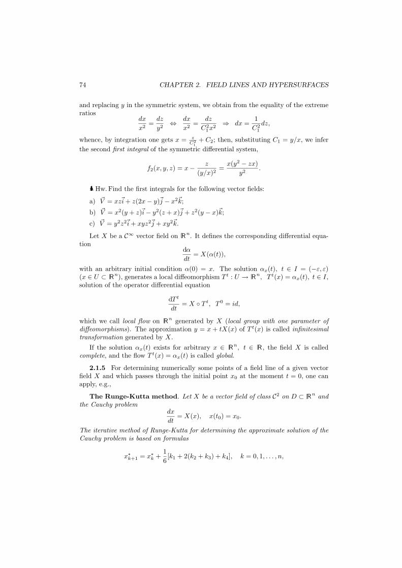
74 CHAPTER 2. FIELD LINES AND HYPERSURFACES
and replacing y in the symmetric system, we obtain from the equality of the extremeratios
dx
x2=
dz
y2⇔ dx
x2=
dz
C21x2
⇒ dx =1
C21
dz,
whence, by integration one gets x = zC2
1+ C2; then, substituting C1 = y/x, we infer
the second first integral of the symmetric differential system,
f2(x, y, z) = x− z
(y/x)2=
x(y2 − zx)y2
.
Hw.Find the first integrals for the following vector fields:
a) ~V = xz~i + z(2x− y)~j − x2~k;
b) ~V = x2(y + z)~i− y2(z + x)~j + z2(y − x)~k;
c) ~V = y2z2~i + xyz2~j + xy2~k.
Let X be a C∞ vector field on Rn. It defines the corresponding differential equa-tion
dα
dt= X(α(t)),
with an arbitrary initial condition α(0) = x. The solution αx(t), t ∈ I = (−ε, ε)(x ∈ U ⊂ Rn), generates a local diffeomorphism T t : U → Rn, T t(x) = αx(t), t ∈ I,solution of the operator differential equation
dT t
dt= X T t, T 0 = id,
which we call local flow on Rn generated by X (local group with one parameter ofdiffeomorphisms). The approximation y = x + tX(x) of T t(x) is called infinitesimaltransformation generated by X.
If the solution αx(t) exists for arbitrary x ∈ Rn, t ∈ R , the field X is calledcomplete, and the flow T t(x) = αx(t) is called global.
2.1.5 For determining numerically some points of a field line of a given vectorfield X and which passes through the initial point x0 at the moment t = 0, one canapply, e.g.,
The Runge-Kutta method. Let X be a vector field of class C2 on D ⊂ Rn andthe Cauchy problem
dx
dt= X(x), x(t0) = x0.
The iterative method of Runge-Kutta for determining the approximate solution of theCauchy problem is based on formulas
x∗k+1 = x∗k +16[k1 + 2(k2 + k3) + k4], k = 0, 1, . . . , n,
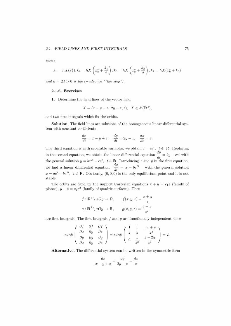
2.1. FIELD LINES AND FIRST INTEGRALS 75
where
k1 = hX(x∗k), k2 = hX
(x∗k +
k1
2
), k3 = hX
(x∗k +
k2
2
), k4 = hX(x∗k + k3)
and h = ∆t > 0 is the t−advance (”the step”).
2.1.6. Exercises
1. Determine the field lines of the vector field
X = (x− y + z, 2y − z, z), X ∈ X (R3),
and two first integrals which fix the orbits.
Solution. The field lines are solutions of the homogeneous linear differential sys-tem with constant coefficients
dx
dt= x− y + z,
dy
dt= 2y − z,
dz
dt= z.
The third equation is with separable variables; we obtain z = cet, t ∈ R . Replacing
in the second equation, we obtain the linear differential equationdy
dt= 2y − cet with
the general solution y = be2t + cet, t ∈ R . Introducing z and y in the first equation,
we find a linear differential equationdx
dt= x − be2t with the general solution
x = aet − be2t, t ∈ R . Obviously, (0, 0, 0) is the only equilibrium point and it is notstable.
The orbits are fixed by the implicit Cartesian equations x + y = c1z (family ofplanes), y − z = c2z
2 (family of quadric surfaces). Then
f : R3 \ xOy → R , f(x, y, z) =x + y
z
g : R3 \ xOy → R , g(x, y, z) =y − z
z2
are first integrals. The first integrals f and g are functionally independent since
rank
∂f
∂x
∂f
∂y
∂f
∂z
∂g
∂x
∂g
∂y
∂g
∂z
= rank
1z
1z
−x + y
z2
01z2
z − 2y
z3
= 2.
Alternative. The differential system can be written in the symmetric form
dx
x− y + z=
dy
2y − z=
dz
z,
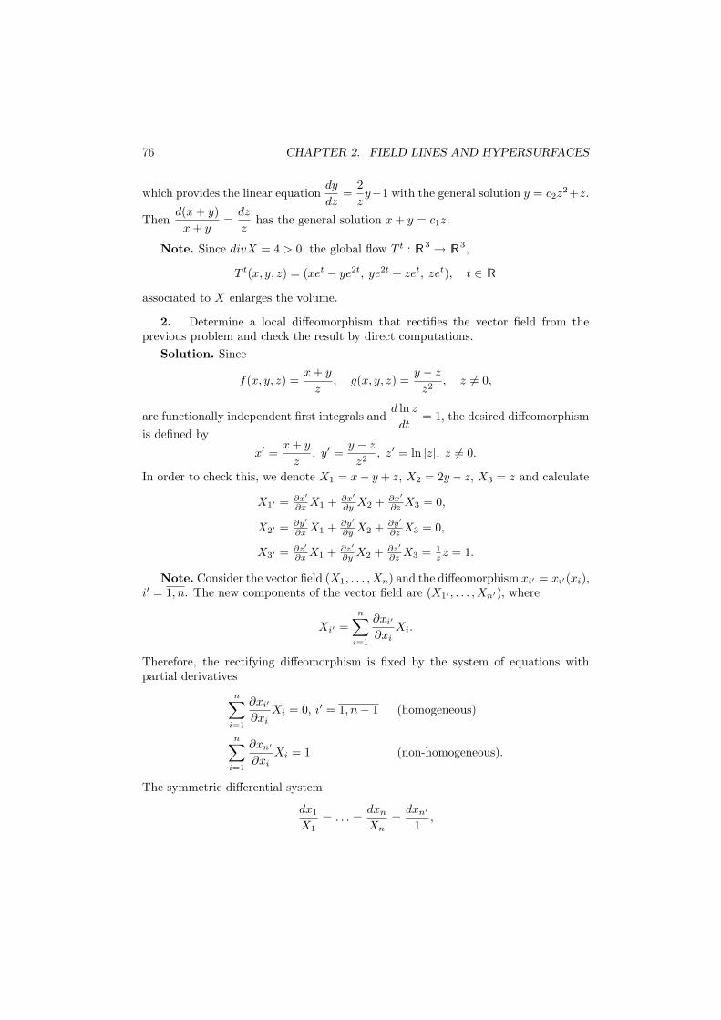
76 CHAPTER 2. FIELD LINES AND HYPERSURFACES
which provides the linear equationdy
dz=
2zy−1 with the general solution y = c2z
2+z.
Thend(x + y)x + y
=dz
zhas the general solution x + y = c1z.
Note. Since divX = 4 > 0, the global flow T t : R3 → R3,
T t(x, y, z) = (xet − ye2t, ye2t + zet, zet), t ∈ R
associated to X enlarges the volume.
2. Determine a local diffeomorphism that rectifies the vector field from theprevious problem and check the result by direct computations.
Solution. Since
f(x, y, z) =x + y
z, g(x, y, z) =
y − z
z2, z 6= 0,
are functionally independent first integrals andd ln z
dt= 1, the desired diffeomorphism
is defined by
x′ =x + y
z, y′ =
y − z
z2, z′ = ln |z|, z 6= 0.
In order to check this, we denote X1 = x− y + z, X2 = 2y − z, X3 = z and calculate
X1′ = ∂x′∂x X1 + ∂x′
∂y X2 + ∂x′∂z X3 = 0,
X2′ = ∂y′
∂x X1 + ∂y′
∂y X2 + ∂y′
∂z X3 = 0,
X3′ = ∂z′∂x X1 + ∂z′
∂y X2 + ∂z′∂z X3 = 1
z z = 1.
Note. Consider the vector field (X1, . . . , Xn) and the diffeomorphism xi′ = xi′(xi),i′ = 1, n. The new components of the vector field are (X1′ , . . . , Xn′), where
Xi′ =n∑
i=1
∂xi′
∂xiXi.
Therefore, the rectifying diffeomorphism is fixed by the system of equations withpartial derivatives
n∑
i=1
∂xi′
∂xiXi = 0, i′ = 1, n− 1 (homogeneous)
n∑
i=1
∂xn′
∂xiXi = 1 (non-homogeneous).
The symmetric differential system
dx1
X1= . . . =
dxn
Xn=
dxn′
1,
2.1. FIELD LINES AND FIRST INTEGRALS 77
assigned to the non-homogeneous equation, shows that x1′ , . . . , x(n−1)′ are the firstintegrals that determine the field lines, and xn′ is determined from
x1′(x1, . . . , xn) = c1, . . . , x(n−1)′(x1, . . . , xn) = cn−1, dxn′ =dxn
Xn(x1, . . . , xn).
3. For each of the following vector fields, determine the field lines by the methodof the integrable combinations and fix a local rectifying diffeomorphism.
a) ~V = xz~i + z(2x− y)~j − x2~k;
b) ~V = x2(y + z)~i− y2(z + x)~j + z2(y − x)~k;
c) ~V = y2z2~i + xyz2~j + xy2z~k;
d) ~V = xz~i + yz~j − (x2 + y2)~k;
e) ~V = (y − z)~i + (z − x)~j + (x− y)~k;
f) ~V = x(y − z)~i + y(z − x)~j + z(x− y)~k.
Solution. a) The symmetric differential system that determines the field lines is
dx
xz=
dy
z(2x− y)=
dz
−x2.
The solutions of the algebraic system xz = 0, z(2x − y) = 0, x2 = 0, i.e., the points(0, y, 0), y ∈ R and (0, 0, z), z ∈ R are equilibrium points of ~V .
The differential equationdx
xz=
dz
−x2is equivalent to xdx + zdz = 0 and has the
general solution defined by x2+z2 = c1 (family of cylindrical surfaces with generatricesparallel to Oy).
We notice that we have
dx
x=
dy
2x− y=
d(x− y)y − x
.
Using either the linear differential equationdy
dx= 2 − 1
xy, or the equation with
separated variablesdx
x=
d(x− y)y − x
, we find x(x − y) = c2 (family of cylindrical
surfaces with the generatrices parallel to Oz).We obtain the field lines (orbits)
x2 + z2 = c1, x(x− y) = c2,
and specify that the Jacobi matrix assigned to the first integrals x2 + z2 and x2 − xyis (
2x 0 2z
2x− y −x 0
).
78 CHAPTER 2. FIELD LINES AND HYPERSURFACES
Hence the first integrals are functionally independent on R3 \ yOz.Since v3 = −x2 = z2 − c1, the rectifying diffeomorphism is defined by
x′ = x2 + z2, y′ = x(x− y), z′ =(∫
dz
z2 − c1
)
c1=x2+z2
.
The function z′ rewrites
z′ =1
2√
c1ln
∣∣∣∣z −√c1
z +√
c1
∣∣∣∣c1=x2+z2
=1
2√
x2 + z2ln
∣∣∣∣∣z −√x2 + z2
z +√
x2 + z2
∣∣∣∣∣ ,
where we neglect the constant of integration that yields just a translation !).
Note. Since div~V = 0 (i.e., ~V is a solenoidal field), the associated flow of ~Vperserves the volume.
b) The symmetric differential system
dx
x2(y + z)=
dy
−y2(z + x)=
dz
z2(y − x)
may be written in the following forms
x−1dx
x(y + z)=
y−1dy
−y(z + x)=
z−1dz
z(y − x)=
x−1dx + y−1dy + z−1dz
0,
x−2dx
y + z=
y−2dy
−z − x=−z−2dz
−y + x=
x−2dx + y−2dy − z−2dz
0.
From x−1dx+ y−1dy + z−1dz = 0 we find xyz = c1 (family of Titeica surfaces), while
from x−2dx+ y−2dy− z−2dz = 0 we obtain1x
+1y− 1
z= c2 (the domain of definition
of the function (first integral) defined by the left side is not connected). Thus, theorbits are depicted by the implicit Cartesian equations
xyz = c1
1x
+1y− 1
z= c2.
To these, we add the equilibrium points which are generated by the solutions of thealgebraic system
x2(y + z) = 0, y2(z + x) = 0, z2(y − x) = 0.
We notice that
v3 = z2(y − x) = z2√
(x + y)2 − 4xy = z2
√(c2 +
1z
)2c21
z2− 4
c1
z.
2.1. FIELD LINES AND FIRST INTEGRALS 79
Therefore the rectifying diffeomorphism is defined by
x′ = xyz, y′ =1x
+1y− 1
z, z′ =
(∫dz√
(zc2 + 1)2c21 − 4c1z3
) ∣∣∣∣ c1 = xyz
c2=1x + 1
y− 1z
(an elliptic antiderivative).
c) From the differential system
dx
dt= y2z2,
dy
dt= xyz2,
dz
dt= xy2z,
we obtain
ydy
dt− z
dz
dt= 0 ⇒ d
dt(y2 − z2) = 0 ⇒ y2 − z2 = c1,
(a family of hyperbolic cylinders with the generatrices parallel to Ox). Moreover, wefind
xdx
dt− y
dy
dt= 0 ⇒ d
dt(x2 − y2) = 0 ⇒ x2 − y2 = c2,
(a family of hyperbolic cylinders with the generatrices parallel to Oz).
It follows that the family of orbits is given by
y2 − z2 = c1
x2 − y2 = c2.
The already determined first integrals are functionally independent on R3 \ (Ox ∪Oy ∪ Oz). The equilibrium points are generated by the solutions of the algebraicsystem
y2z2 = 0, xyz2 = 0, xy2z = 0.
We can writev3 = xy2z =
√c1 + c2 + z2(c1 + z2)z,
function that determines the rectifying diffeomorphism
x′ = y2 − z2, y′ = x2 − y2, z′ =(∫
dz√c1 + c2 + z2(c1 + z2)z
) ∣∣∣∣ c1=y2−z2
c2=x2−y2
.
Note. We can write ~V = yz grad (xyz), that is, ~V is a bi-scalar vector field.
d) Consider the first-order differential system
dx
dt= xz,
dy
dt= yz,
dz
dt= −x2 − y2.
80 CHAPTER 2. FIELD LINES AND HYPERSURFACES
We notice that the axis Oz consists of equilibrium points. Then,
d
dtln |x| = d
dtln |y|, x 6= 0, y 6= 0
implies x = c1y, x 6= 0, y 6= 0 (family of parts of planes). By analogy,
xdx
dt+ y
dy
dt+ z
dz
dt= 0
givesd
dt(x2 + y2 + z2) = 0 or x2 + y2 + z2 = c2,
a family of spheres of centre at the origin. All in all, the orbits are arcs of circles(which may degenerate in particular to points).
Fromx = c1y, x2 + y2 + z2 = c2, v3 = −x2 − y2,
we find v3 = z2 − c2. Thus,
x′ =x
y, y′ = x2 + y2 + z2,
z′ =∫
dz
z2 − c2
∣∣∣∣c2=x2+y2+z2
=1
2√
c2ln
∣∣∣∣z −√c2
z +√
c2
∣∣∣∣c2=x2+y2+z2
=
=1
2√
x2 + y2 + z2ln
∣∣∣∣∣z −
√x2 + y2 + z2
z +√
x2 + y2 + z2
∣∣∣∣∣ ,
where we neglected the constant of integration, define a rectifying diffeomorphism.
Note. The vector ~V =z3
2grad
x2 + y2
z2, z 6= 0 is a bi-scalar vector field.
e) The homogeneous differential linear system
dx
dt= y − z,
dy
dt= z − x,
dz
dt= x− y
admits a straight line of equilibrium points of equations x = y = z. We also infer
dx
dt+
dy
dt+
dz
dt= 0 ⇒ x + y + z = c1
xdx
dt+ y
dy
dt+ z
dz
dt= 0 ⇒ x2 + y2 + z2 = c2,
which represent respectively a family of planes and a family of spheres.
Hence the orbits are circles laying in planes which are perpendicular to the straightline x = y = z. f) Hw.
2.1. FIELD LINES AND FIRST INTEGRALS 81
4. For each of the following vector fields, determine the field lines and fix a localrectifying diffeomorphism:
a) ~V = (x2 − y2 − z2)~i + 2xy~j + 2xz~k;
b) ~V = x~i + y~j + (z +√
x2 + y2 + z2)~k;
c) ~V = (x− y)~i + (x + y)~j + z~k;
d) ~V = (x + y)~i− x(x + y)~j + (x− y)(2x + 2y + z)~k;
e) ~V = x~i + y~j + (z − x2 − y2)~k;
f) ~V = y~i + x~j + 2xy√
a2 − z2~k;
g) ~V = (x2 − yz)~i + (y2 − zx)~j + (z2 − xy)~k;
h) ~V = (xy − 2z2)~i + (4xz − y2)~j + (yz − 2x2)~k.In each case, find the field line that passes through the point (1,1,1).
Hint. The field lines are: a) y = c1z, x2 + y2 + z2 = 2c2z,
b) y = c1x, z = c2 +√
x2 + y2 + z2;
c)dz
z=
12
d(x2 + y2)x2 + y2
=d(x−1y)
1 + (x−1y)2;
d) x2 + y2 = c1, (x + y)(x + y + z) = c2;e) y = c1x, z + x2 + y2 = c2x;
f) x2 − y2 = c1, x2 + y2 = 2arcsinz
a+ c2;
g) x− y = c1(y − z), xy + yz + zx = c2;h) z2 + xy = c1, x2 + yz = c2.
5. Determine the vector fields whose orbits are
a)
x + arcsiny
z= c1
y + arcsinx
z= c2,
b)
cosh xy + z = c1
x + sinh yz = c2.
6. Approximate the solution of the Cauchy problem
dx
dt= x(1− 2y2),
dy
dt= −y(1 + 2x2),
dz
dt= 2z(x2 + y2),
x(0) = y(0) = z(0) = 1, t ∈ [0, 10], h = 0.2,
by the Runge-Kutta method. Verify the result using first integrals.
7. Study the completeness of the vector fields from the problem 4.
82 CHAPTER 2. FIELD LINES AND HYPERSURFACES
8. Consider the Hamiltonian
H(x, y) =12
3∑
k=1
y2k + V (x).
In each of the following cases determine the flow generated by the Hamiltonian vectorfield associated to H and specify if it is a global flow.
a) V (x) = x21 − x2
2 + x3,b) V (x) = x2
1 + x2 + x3,
Solution. a) We obtain
x1 = a1 cos√
2t + b1 sin√
2t
x2 = a2e√
2t + b2e−√2t
x3 = −12t2 + a3t + b3
;
y1 =√
2a1 sin√
2t− 2b1 cos√
2t
y2 = −√2a2e√
2t + 2b2e−√2t
y3 = t− a3,
t ∈ R (global flow).
9. In each of the following cases, determine the infinitesimal transformation andthe flow generated by the vector field X. Study if the corresponding flow reduces,enlarges or preserves the volume and specify the fixed points.
a) X = (−x(x2 + 3y2),−2y3,−2y2z);b) X = (3xy2 − x3,−2y3,−2y2z);c) X = (xy2, x2y, z(x2 + y2));d) X = (x(y2 − z2),−y(x2 + z2), z(x2 + y2));e) X = (x(y − z), y(z − x), z(x− y));f) X = ((z − y)2, z, y).Hint. a) and b) reduce the volume; c) and d) enlarge the volume; e) and f)
preserve the volume.
2.2 Field hypersurfaces and linear PDEs
2.2.1 Let D ⊂ Rn be an open and connected subset, and let X be a vector fieldof class C1 on D of components (X1, . . . , Xn), Xi : D → R , i = 1, n. For a givenfunction f : D → R of class C1 and for C ∈ R , the set of constant level
M : f(x1, . . . , xn) = C
determines a hypersurface of Rn iff
grad f |M 6= 0.
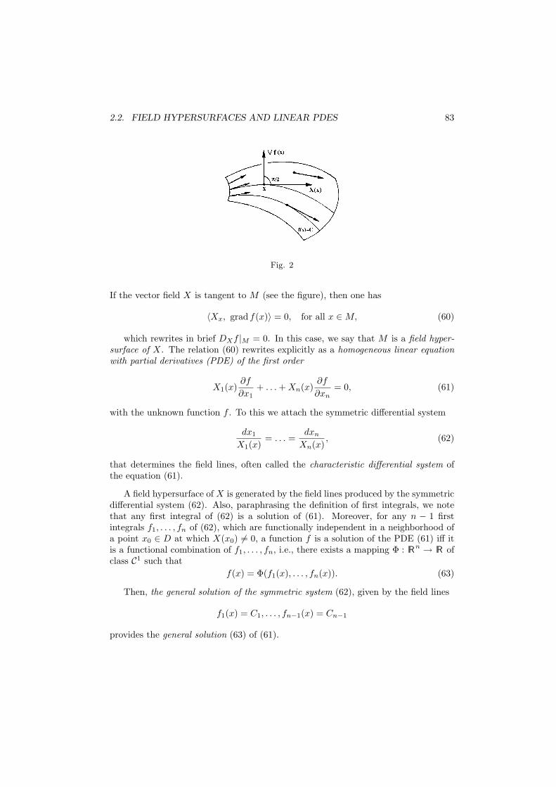
2.2. FIELD HYPERSURFACES AND LINEAR PDES 83
Fig. 2
If the vector field X is tangent to M (see the figure), then one has
〈Xx, grad f(x)〉 = 0, for all x ∈ M, (60)
which rewrites in brief DXf |M = 0. In this case, we say that M is a field hyper-surface of X. The relation (60) rewrites explicitly as a homogeneous linear equationwith partial derivatives (PDE) of the first order
X1(x)∂f
∂x1+ . . . + Xn(x)
∂f
∂xn= 0, (61)
with the unknown function f . To this we attach the symmetric differential system
dx1
X1(x)= . . . =
dxn
Xn(x), (62)
that determines the field lines, often called the characteristic differential system ofthe equation (61).
A field hypersurface of X is generated by the field lines produced by the symmetricdifferential system (62). Also, paraphrasing the definition of first integrals, we notethat any first integral of (62) is a solution of (61). Moreover, for any n − 1 firstintegrals f1, . . . , fn of (62), which are functionally independent in a neighborhood ofa point x0 ∈ D at which X(x0) 6= 0, a function f is a solution of the PDE (61) iff itis a functional combination of f1, . . . , fn, i.e., there exists a mapping Φ : Rn → R ofclass C1 such that
f(x) = Φ(f1(x), . . . , fn(x)). (63)
Then, the general solution of the symmetric system (62), given by the field lines
f1(x) = C1, . . . , fn−1(x) = Cn−1
provides the general solution (63) of (61).
84 CHAPTER 2. FIELD LINES AND HYPERSURFACES
2.2.2 Example. Consider the homogeneous linear PDE:
(x− a)∂f
∂x+ (y − b)
∂f
∂y+ (z − c)
∂f
∂z= 0.
The associated symmetric differential system
dx
x− a=
dy
y − b=
dz
z − c
admits the first integrals (obtained from the ODE provided by both the equalities)
f1(x, y, z) =x− a
y − b, f2(x, y, z) =
y − b
z − c.
Hence the field lines of the field X(x, y, z) = (x − a, y − b, z − c) are given by thetwo-parameter family of curves
f1 = C1
f2 = C2⇔
x− a
y − b= C1
y − b
z − c= C2
⇔
x− a− C1(y − b) = 0y − b− C2(z − c) = 0,
i.e., a family of straight lines in R3. Moreover, the first integrals f1 and f2 providethe general solution f of the form
f(x, y, z) = Φ(
x− a
y − b,y − b
z − c
),
with arbitrary function Φ : R2 → R of class C1.
2.2.3 Let f = (f1, . . . , fn−1) be the general solution of the system (62), and
MC : Φ(f1(x), . . . , fn−1(x)) = 0
the associated family of field hypersurfaces. For determining a unique solution of (61),(i.e., a determined hypersurface M0 : Φ(f1(x), . . . , fn−1(x)) = 0 attached to X) oneneeds to impose certain restrictive conditions besides (61). This leads to
The Cauchy problem for the linear homogeneous PDE. Find the field
hypersurface which contains the submanifold with n−2 dimensions Γ :
g(x) = 0h(x) = 0
(see the figure).
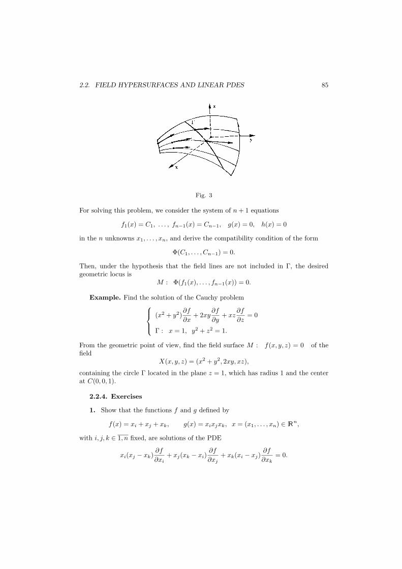
2.2. FIELD HYPERSURFACES AND LINEAR PDES 85
Fig. 3
For solving this problem, we consider the system of n + 1 equations
f1(x) = C1, . . . , fn−1(x) = Cn−1, g(x) = 0, h(x) = 0
in the n unknowns x1, . . . , xn, and derive the compatibility condition of the form
Φ(C1, . . . , Cn−1) = 0.
Then, under the hypothesis that the field lines are not included in Γ, the desiredgeometric locus is
M : Φ(f1(x), . . . , fn−1(x)) = 0.
Example. Find the solution of the Cauchy problem
(x2 + y2)∂f
∂x+ 2xy
∂f
∂y+ xz
∂f
∂z= 0
Γ : x = 1, y2 + z2 = 1.
From the geometric point of view, find the field surface M : f(x, y, z) = 0 of thefield
X(x, y, z) = (x2 + y2, 2xy, xz),
containing the circle Γ located in the plane z = 1, which has radius 1 and the centerat C(0, 0, 1).
2.2.4. Exercises
1. Show that the functions f and g defined by
f(x) = xi + xj + xk, g(x) = xixjxk, x = (x1, . . . , xn) ∈ Rn,
with i, j, k ∈ 1, n fixed, are solutions of the PDE
xi(xj − xk)∂f
∂xi+ xj(xk − xi)
∂f
∂xj+ xk(xi − xj)
∂f
∂xk= 0.
86 CHAPTER 2. FIELD LINES AND HYPERSURFACES
Solution. We notice that
∂f
∂xi= 1,
∂f
∂xj= 1,
∂f
∂xk= 1,
∂f
∂xl= 0, l 6= i, j, k,
and∂g
∂xi= xjxk,
∂g
∂xj= xixk,
∂g
∂xk= xixj ,
∂g
∂xl= 0, l 6= i, j, k.
Introducing these relations in the equations, we obtain identities.
2. Let the vector fields
X1 = (1, 0, 0), X2 = (0, 1, 0), X3 = (0, 0, 1),
X4 = (−x2, x1, 0), X5 = (0,−x3, x2), X6 = (x3, 0,−x1), (x1, x2, x3) ∈ R3
be linearly independent Killing vector fields in X (R3). Determine the field surfacesof these fields.
Solution. A vector field X = (X1, . . . , Xn) on Rn that satisfies the system with
partial derivatives∂Xi
∂xj+
∂Xj
∂xi= 0, i, j = 1, . . . , n is called a Killing field.
Taking account of the definition of the field hypersurfaces, we write the homoge-neous linear PDEs of the first order and find their solutions.
We get∂f
∂x1= 0 ⇒ f1(x2, x3) = c1 (families of cylindrical surfaces with genera-
trices parallel to Ox2). By cyclic permutations, we get the field surfaces of X2 andX3 as being f2(x3, x1) = c2 (families of cylindrical surfaces with generatrices parallelto Ox2) respectively f3(x1, x2) = c3 (families of cylindrical surfaces with generatricesparallel to Ox1).
For X4 we obtain −x2∂f
∂x1+ x1
∂f
∂x2= 0. To this equation, we assign the char-
acteristic differential systemdx1
−x2=
dx2
x1=
dx3
0and the general solution of the
equation with partial derivatives is f4(x21 + x2
2, x3) = c4 (families of surfaces of revo-lution). By circular permutations, we find other two families of surfaces of revolutionf5(x2
2 + x23, x1) = c5 and f6(x2
3 + x21, x2) = c6 corresponding to X5, respectively, X6.
3. For each of the following vector fields, determine the family of their fieldsurfaces.
a) ~V = x(x + z)~i + y(y + z)~j + (z2 − xy)~k,
b) ~V = (xy3 − 2x4)~i + (2y4 − x3y)~j + 9z(x3 − y3)~k,
c) ~V = (x2 + y2)~i + 2xy~j + xz~k.
Solution. a) To the equation
x(x + z)∂f
∂x+ y(y + z)
∂f
∂y+ (z2 − xy)
∂f
∂z= 0,
2.2. FIELD HYPERSURFACES AND LINEAR PDES 87
we assign the symmetric differential system
dx
x(x + z)=
dy
y(y + z)=
dz
z2 − xy.
Fromdx
x(x + z)=
ydz − zdy
−y2(x + z)it follows
dx
x= −ydz − zdy
y2, and then ln |x|+ z
y= c1
(the domain of definition of the first integral (x, y, z) → ln |x|+ z
yis not connected).
Fromdy
y(y + z)=
xdz − zdx
−x2(y + z), we find
dy
y= −xdz − zdx
x2and hence ln |y|+ z
x= c2.
The family of orbits
ln |x|+ z
y= c1, ln |y|+ z
x= c2, x 6= 0, y 6= 0
produces the family of the field surfaces
Φ(
ln |x|+ z
y, ln |y|+ z
x
)= 0, x 6= 0, y 6= 0,
where Φ is an arbitrary function of class C1, and f = Φ(c1, c2).
Note. It remains to find the field lines on x = 0, y 6= 0. The restriction of ~V tox = 0, y 6= 0 is
~V (0, y, z) = y(y + z)~j + z2~k.
Fromdy
y(y + z)=
dz
z2, we obtain
dz
dy=
z2
y(y + z)(homogeneous differential equation)
with the general solution z = c3e−z/y. Then x = 0, z = c3e
−z/y are field lines of ~V .
By analogy, we discuss the cases x 6= 0, y = 0, respectively x = 0, y = 0.
The equation
(xy3 − 2x4)∂f
∂x+ (2y4 − x3y)
∂f
∂y+ 9z(x3 − y3)
∂f
∂z= 0
corresponds to the characteristic system
dx
xy3 − 2x4=
dy
2y4 − x3y=
dz
9z(x3 − y3).
We notice that 3x2y3zdx + 3x3y2zdy + x3y3dz = 0 and thus x3y3z = c1. Then, wesee that
(y−2 − 2x−3y)dx + (x−2 − 2y−3)dy = 0
and so xy−2 + yx−2 = c2 (the domain of definition of this first integral, characterizedby x 6= 0, y 6= 0, is not connected).
88 CHAPTER 2. FIELD LINES AND HYPERSURFACES
The family of surfaces that contains the family of orbits
x3y3z = c1, xy−2 + x−2y = c2, x 6= 0, y 6= 0
has the equation
Φ(x3y3z, xy−2 + x−2y) = c, x 6= 0, y 6= 0,
where Φ is an arbitrary function of class C1.
Note. a) For x = 0, y 6= 0 we find ~V (0, y, z) = 2y4~j − 9zy3~k. The differential
equationdy
2y4=
dz
−9zy3has the general solution y9z2 = c3. Hence the field lines are
x = 0, y9z2 = c3.
By analogy, we treat the case x 6= 0, y = 0.
b) The relation Φ(x3y3z, xy−2 + x−2y) = c rewrites x3y3z = ϕ(xy−2 + x−2y),where ϕ is an arbitrary function of class C1.
c) To the equation
(x2 + y2)∂f
∂x+ 2xy
∂f
∂y+ xz
∂f
∂z= 0
we associate the symmetric differential system
dx
x2 + y2=
dy
2xy=
dz
zx.
We inferdy
y= 2
dz
z⇒ z2 = c1y
d(x− y)(x− y)2
=d(x + y)(x + y)2
⇒ x2 − y2 = c2y.
Hence the family of the field surfaces has the equation
Φ(
z2
y,x2 − y2
y
)= c,
y 6= 0, where Φ is an arbitrary function of class C1.
For y = 0, we obtain ~V (x, 0, z) = x2~i + xz~k, anddx
x2=
dz
xzyields x = c3z, z 6= 0.
Thus, y = 0, x = c3z; z 6= 0 are field lines.
4. Consider the vector field
~V = x2(y + z)~i− y2(x + z)~j + z2(y − x)~k.
2.3. NONHOMOGENEOUS LINEAR PDES 89
Determine the field surface that passes through the curve of equations
xy = 1x + y = 1.
Solution. We notice that
dx
x2(z + y)=
dy
−y2(z + x)=
dz
z2(y − x)=
=x−1dx + y−1dy + z−1dz
0=
x−2dx + y−2dy − z−2dz
0.
Then the family of orbits of ~V is
xyz = c1
1x
+1y− 1
z= c2, x 6= 0, y 6= 0, z 6= 0.
(64)
The condition of compatibility of the system
xyz = c1, xy = 1, y + x = 1,
1x
+1y− 1
z= c2, x 6= 0, y 6= 0, z 6= 0,
selects the orbits which lean upon the given curve. We find 1 − c−11 = c2. We
reconsider the desired surface as being the locus of the orbits (64) which satisfy thecondition 1− c−1
1 = c2. Eliminating the parameters c1, c2, we obtain the surface
1− 1xyz
=1x
+1y− 1
z, x 6= 0, y 6= 0, z 6= 0.
Note. div ~V = 0, and hence ~V is a solenoidal field.
2.3 Nonhomogeneous linear PDEs
2.3.1 Definition. We call nonhomogeneous linear equation with partial derivativesof order one, a PDE with unknown function f : D ⊂ Rn → R of the form
X1(x, f(x))∂f
∂x1+ . . . + Xn(x, f(x))
∂f
∂xn= F (x, f(x)),
where X1, . . . , Xn, F : Rn+1 → R are differentiable functions of class C1.
For solving this type of PDE, we look for the solution f given in implicit formΦ(x, f) = 0, provided by a PDE of form (61) with the associated symmetric differentialsystem
dx1
X1(x, f)= . . .
dxn
Xn(x, f)=
df
F (x, f).
90 CHAPTER 2. FIELD LINES AND HYPERSURFACES
2.3.2 Example. Find the general solution of the PDE
xz∂z
∂x− yz
∂z
∂y= x2 + y2.
Solution. The characteristic symmetric differential system is
dx
xz=
dy
−yz=
dz
x2 + y2.
Its first integrals are
f1(x, y, z) = xy, f2(x, y, z) = (x2 − y2 + z2)/2,
hence the general solution is given implicitly by equation of the form
Φ(xy, (x2 − y2 + z2)/2) = 0.
2.3.3. Exercises
1. Solve the following Cauchy problems
a) z(x + z)∂z
∂x− y(y + z)
∂z
∂y= 0, z(1, y) =
√y;
b)∂z
∂y= xz
∂z
∂x, z(x, 0) = x.
Solution. a) This is a non-homogeneous linear equation with partial derivativesof the first order. The associate symmetric differential system is
dx
z(x + z)=
dy
−y(y + z)=
dz
0,
and dz = 0 implies z = c1. Then the system rewrites
dy
y(y + c1)=
−dx
−c1(x + c1)⇔ 1
y(y + c1)=
1c1y
− 1c1(y + c1)
,
whencey(x + c1)
y + c1= c2 and after plugging in c1 = z, we find
y(x + z)y + z
= c2.
The general solution of the equation with partial derivatives isy(x + z)
y + z= ϕ(z),
where ϕ is an arbitrary function of class C1. Putting the condition z(1, y) =√
y, it
followsy(1 +
√y)
y +√
y= ϕ(
√y) or, otherwise, ϕ(u) =
u2(1 + u)u2 + u
= u. Coming back to
the general solution, we findy(x + z)
y + z= z or z =
√xy.
2.3. NONHOMOGENEOUS LINEAR PDES 91
b) Non-homogeneous linear equation with partial derivatives of the first order.
The characteristic differential systemdx
−xz=
dy
1=
dz
0becomes z = c1,
dx
x= −c1dy
or z = c1, x = c2e−yz.
The general solution of the equation with partial derivatives is z = Φ(xeyz), whereΦ is an arbitrary function of class C1. Putting the condition z(x, 0) = x, we findΦ(x) = x, or otherwise, Φ(u) = u. Coming back with this function Φ in the generalsolution, we obtain z = xeyz.
2. Determine the general solution of the Euler equation
n∑
i=1
xi∂f
∂xi(x) = pf(x).
Solution. Assuming p 6= 0, the characteristic system
dx1
x1= . . . =
dxn
xn=
df
pf
admits the general solution
x2 = c1x1, x3 = c2x1, . . . , xn = cn−1x1, f = cnxp1.
The general solution of the Euler equation is the homogeneous function
f(x) = xp1ϕ
(x2
x1, . . . ,
xn
x1
),
where ϕ is a function of class C1; we note that f has the degree of homogeneity p.
3. Let there be given the vector fields
X = (y,−x, 0), Y = (x, y,−z), Z = (x2, yx, xz), U = (xy, y2, yz), V = (xz, yz, z2).
Show that the family of conesx2 + y2 = c2z2,
where c is a real parameter, is invariant with respect to the flow generated by each ofthe given vector fields.
Solution. Consider the function f : R3 \ xOy → R , f(x, y, z) = x2+y2
z2 .We find
DXf = y∂f
∂x− x
∂f
∂y= y
2x
z2− x
2y
z2= 0,
DY f = x∂f
∂x+ y
∂f
∂y− z
∂f
∂z= x
2x
z2+ y
2y
z2− z
2(x2 + y2)z3
= 0,
DZf = 0, DUf = 0, DV f = 0.
92 CHAPTER 2. FIELD LINES AND HYPERSURFACES
Note. f is a first integral that is common to all the systems that determine the fieldlines of X, Y, U, Z and respectively V .
4. Determine the implicit Cartesian equation of the cylinder with generatricesparallel to ~V =~i+~j−~k and having as a director curve the circle C : x2+y2 = 1, z = 1.
Solution. We have to solve the following Cauchy problem: determine the fieldsurface of ~V that leans upon the circle C. The equation
∂f
∂x+
∂f
∂y− ∂f
∂z= 0
has the characteristic systemdx
1=
dy
1=
dz
−1,
with the general solution y−x = c1, z +x = c2. Among these straight lines, we selectthose which lean upon the circle C, that is, we find the condition of compatibility ofthe system
y − x = c1, z + x = c2, x2 + y2 = 1, z = 1.
We reconsider the desired surface as being the locus of the straight lines y − x = c1,z + x = c2 which satisfy
(c2 − 1)2 + (c2 + c1 − 1)2 = 1.
After replacing c1, c2 with the corresponding first integrals, we get
(z + x− 1)2 + (z + y − 1)2 = 1.
5. Determine the implicit Cartesian equation of the cone that has the vertex atthe origin of the axes and the director curve C : x2 + y2 = x, z = 1.
Solution. The concurrent vector field determined by O(0, 0, 0) and M(x, y, z) isX = (x, y, z). By this notice, we get a Cauchy problem: determine the field surfaceof X that leans upon the circle C. The field surfaces of X are the sets of constantlevel assigned to the solutions of the PDE
x∂f
∂x+ y
∂f
∂y+ z
∂f
∂z= 0.
To this, it corresponds the characteristic system
dx
x=
dy
y=
dz
z
with the general solution y = c1x, z = c2x.The condition of compatibility of the algebraic system
y = c1x, z = c2x, x2 + y2 = x, z = 1
2.3. NONHOMOGENEOUS LINEAR PDES 93
is 1 + c21 = c2. Plugging in c1 = y/x, c2 = z/x in this relation, we find
1 +y2
x2=
z
x⇔ x2 + y2 = zx.
6. Determine the implicit Cartesian equation of the surface obtained by therotation of the parabola P : y2 = 2z + 1, x = 0 about the axis Oz.
Solution. Consider the vector field ~X = x~i + y~j + z~k and y = ~k the parallelvector field that gives the direction of the axis. It follows the Killing vector field~Z = ~X × ~Y = y~i − x~j. By this remark, it remains to find the field surface of ~Zthat leans upon the parabola P . We find the orbits of ~Z, that is, the solutions of thesystem
dx
y=
dy
−x=
dz
0.
These are z = c1, x2 +y2 = c2 (family of circles). We select the circles that lean uponP ; the condition of compatibility of the algebraic system
z = c1, x2 + y2 = c2, y2 = 2z + 1, x = 0
is c2 = 2c1 + 1. We consider the surface as being the locus of the circles z = c1,x2 + y2 = c2 for which c2 = 2c1 + 1. Eliminating c1, c2 we find the paraboloid
x2 + y2 − 2z = 1.
7. There are given the following vector fields:
X = (1, 2x, 3y), Y = (x, 2y, 3z), Z = (0, 1, 3x)
and the function f : R3 → R , f(x, y, z) = 3xy − z − 2x3. Show that:
a) the function f is invariant with respect to the groups of one parameter generatedby X, respectively Z;
b) the function f is a eigenvector of Y with respect to the eigenvalue 3.
Solution. a) By direct computation, we yield
DXf =∂f
∂x+ 2x
∂f
∂y+ 3y
∂f
∂z= 3y − 6x2 + 2x · 3x + 3y(−1) = 0
DZf =∂f
∂y+ 3x
∂f
∂z= 0.
b) DY f = x∂f
∂x+ 2y
∂f
∂y+ 3z
∂f
∂z= x(3y − 6x2) + 6xy − 3z = 3f .
8. Let x = (x1, x2, x3, x4) ∈ R4. Verify that the function defined by
f(x) =x1 − x3
x1 − x4
x2 − x4
x2 − x3

94 CHAPTER 2. FIELD LINES AND HYPERSURFACES
is a solution of the PDEs
4∑
i=1
∂f
∂xi= 0,
4∑
i=1
xi∂f
∂xi= 0,
4∑
i=1
x2i
∂f
∂xi= 0.
9. For each of the following vector fields, determine the family of the field surfaces.
a) ~V = 2(x2 − y2)~i + 2xy~j + xyz~k;
b) ~V = (z + ex)~i + (z + ey)~j + (z2 − ex+y)~k;
c) ~V = xy~i− y√
1− y2~j + (z√
1− y2 − 2axy)~k.
Hint. We obtain: a) z2 = eyϕ(y2ex2/y2), b) y + ze−x = ϕ(x + ze−y),
c) yz + ax(y +√
1− y2) = ϕ(xearcsin y).
10. Consider the vector field ~V = xz~i + z(2x − y)~j − x2~k. Determine the fieldsurface containing the curve xy = 1, xz = 1.
11. Solve the following Cauchy problems:
a) x∂z
∂y− y
∂z
∂x= 0, z(x, 0) = ϕ(x);
b)∂z
∂x+
∂z
∂y= z2, z(x, 0) = ψ(x);
c) x∂f
∂x+ y
∂f
∂y+
∂f
∂z= f, f(x, y, 0) = χ(x).
Hint. a) z = ϕ(√
x2 + y2), b) z =ψ(x− y)
1− yψ(x− y), c) f = χ(xe−z, ye−z)ez.
12. Show that the harmonic polynomials of two variables are homogeneouspolynomials.
Hint. (x + iy)n = Pn(x, y) + iQn(x, y) implies
∂Pn
∂x= nPn−1,
∂Pn
∂y= −nQn−1,
∂Qn
∂x= nQn−1,
∂Qn
∂y= nPn−1,
Pn+1 = xPn − yQn, Qn+1 = yPn + xQn,
and hencex
∂Pn
∂x+ y
∂Pn
∂y= nPn, x
∂Qn
∂x+ y
∂Qn
∂y= nQn.
13. Let f : R2n → R , (x, y) → f(x, y) be a function of class C∞ on R2n\Rn,where Rn = (x, y) ∈ R2n|y = 0. Show that if f(x, 0) = 0 and if the partial
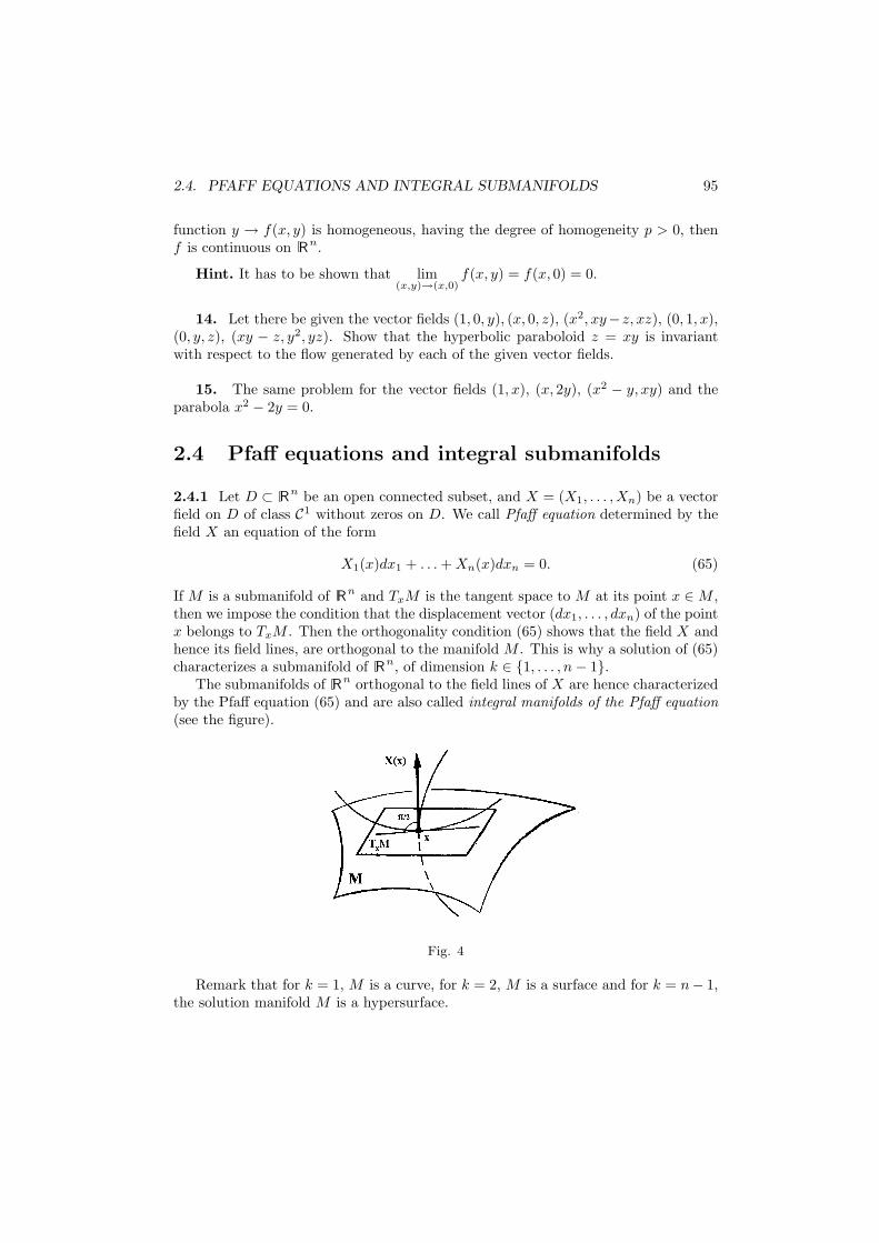
2.4. PFAFF EQUATIONS AND INTEGRAL SUBMANIFOLDS 95
function y → f(x, y) is homogeneous, having the degree of homogeneity p > 0, thenf is continuous on Rn.
Hint. It has to be shown that lim(x,y)→(x,0)
f(x, y) = f(x, 0) = 0.
14. Let there be given the vector fields (1, 0, y), (x, 0, z), (x2, xy−z, xz), (0, 1, x),(0, y, z), (xy − z, y2, yz). Show that the hyperbolic paraboloid z = xy is invariantwith respect to the flow generated by each of the given vector fields.
15. The same problem for the vector fields (1, x), (x, 2y), (x2 − y, xy) and theparabola x2 − 2y = 0.
2.4 Pfaff equations and integral submanifolds
2.4.1 Let D ⊂ Rn be an open connected subset, and X = (X1, . . . , Xn) be a vectorfield on D of class C1 without zeros on D. We call Pfaff equation determined by thefield X an equation of the form
X1(x)dx1 + . . . + Xn(x)dxn = 0. (65)
If M is a submanifold of Rn and TxM is the tangent space to M at its point x ∈ M ,then we impose the condition that the displacement vector (dx1, . . . , dxn) of the pointx belongs to TxM . Then the orthogonality condition (65) shows that the field X andhence its field lines, are orthogonal to the manifold M . This is why a solution of (65)characterizes a submanifold of Rn, of dimension k ∈ 1, . . . , n− 1.
The submanifolds of Rn orthogonal to the field lines of X are hence characterizedby the Pfaff equation (65) and are also called integral manifolds of the Pfaff equation(see the figure).
Fig. 4
Remark that for k = 1, M is a curve, for k = 2, M is a surface and for k = n− 1,the solution manifold M is a hypersurface.
96 CHAPTER 2. FIELD LINES AND HYPERSURFACES
The integral manifold M can be described as follows:
• by an immersion f = (f1, . . . , fn), f(u) = (f1(u), . . . , fn(u)), u = (u1, . . . , uk),subject to the condition of orthogonality
X1(f(u))∂f1
∂uj+ . . . + Xn(f(u))
∂fn
∂uj= 0, j = 1, k;
• by a submersion F = (F1, . . . , Fn−k),
M :
F1(x) = 0. . .Fn−k(x) = 0,
subject to the condition that (65) is a consequence of the relations
F1(x) = 0, . . . , Fn−k(x) = 0
dF1 = 0, . . . , dFn−k = 0.
2.4.2 The integral curves of the Pfaff equation are characterized by the differentialequation
X1(α(t))dx1
dt+ . . . + Xn(α(t))
dxn
dt= 0.
2.4.3 Theorem. Let X = (X1, . . . , Xn) be a vector field which satisfies thecondition
∂Xi
∂xj=
∂Xj
∂xi, for all i, j = 1, n
(i.e., is an irrotational vector field), and x0 = (x10, . . . , xn0) ∈ Rn.
a) If D is an n−dimensional interval (i.e., a Cartesian product of n intervals),then the level hypersurfaces of the function
f : D → R , f(x) =n∑
i=1
∫ xi
xi0
Xi(x10, . . . , xi−10, xi, . . . , xn)dxi
are orthogonal to the field X, and hence the integral hypersurfaces of the Pfaff equation(65).
b) If D is a convex set, then the level hypersurfaces of
f(x) =∫ 1
0
〈X(x0+t(x−x0)), x− x0〉dt
are integral hypersurfaces of the Pfaff equation (65).
2.4. PFAFF EQUATIONS AND INTEGRAL SUBMANIFOLDS 97
Remark. Since X is irrotational, it is locally a potential vector field, i.e., thereexists a function f such that X = grad f .
The Pfaff equation (65) is said to be an exact equation if there exists a functionf : D → R of class C2 such that
∂f
∂xi(x) = Xi(x), i = 1, n,
or, equivalently,
df(x) =n∑
i=1
Xi(x)dxi.
If the Pfaff equation (65) is not exact, sometimes there exists a non-constantfunction µ : D → R \ 0 of class C1 such that
µ(x)X1(x)dx1 + . . . + µ(x)Xn(x)dxn = 0
is an exact equation; in this case the function µ is called an integrant factor and itsatisfies the system with partial derivatives
∂(µXi)∂xj
(x) =∂(µXj)
∂xi(x), i, j = 1, n; i 6= j.
The existence of an integrant factor implies the existence of a function λ such thatX = λ grad f .
The locally exact Pfaff equations and those Pfaff equations which admit a localintegrant factor are called completely integrable equations. The Pfaff equation (65) iscompletely integrable if and only if through each point x0 ∈ D, it passes an integralhypersurface of the equation.
The set of all the integral hypersurfaces of a completely integrable Pfaff equationis called the general solution of the equation.
2.4.4 For n = 2, the Pfaff equation (65) is completely integrable. For n ≥ 3, thePfaff equation (65) is completely integrable if and only if
Xi
(∂Xk
∂xj− ∂Xj
∂xk
)+ Xj
(∂Xi
∂xk− ∂Xk
∂xi
)+ Xk
(∂Xj
∂xi− ∂Xi
∂xj
)= 0, i, j, k = 1, n.
2.4.5 Let X be a vector field of class C1 on a domain D ⊂ Rn. We assume thatthere exist two scalar fields λ of class C1 and f of class C2 such that X = λ grad f .If λ and f are functionally independent, then X is called a bi-scalar field. If λ and fare functionally dependent, then X is a potential field.
X is locally bi-scalar or locally potential vector field if and only if it admits a familyof hypersurfaces of constant level orthogonal to the field lines (see the figure).
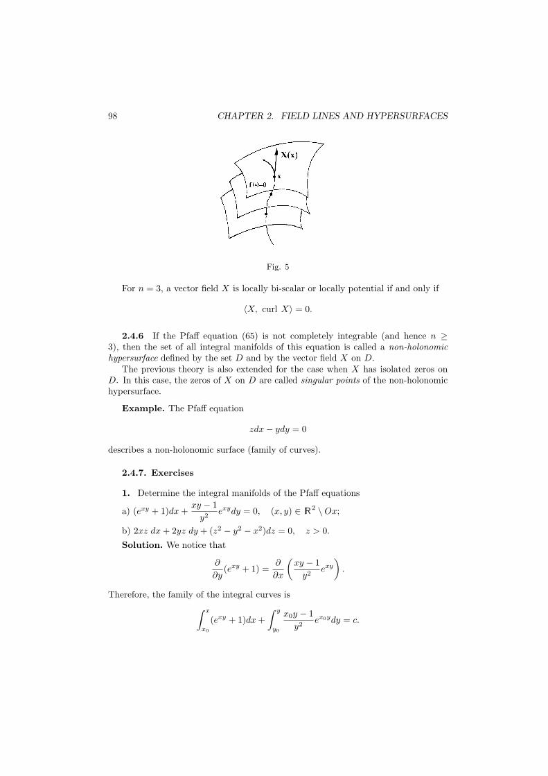
98 CHAPTER 2. FIELD LINES AND HYPERSURFACES
Fig. 5
For n = 3, a vector field X is locally bi-scalar or locally potential if and only if
〈X, curl X〉 = 0.
2.4.6 If the Pfaff equation (65) is not completely integrable (and hence n ≥3), then the set of all integral manifolds of this equation is called a non-holonomichypersurface defined by the set D and by the vector field X on D.
The previous theory is also extended for the case when X has isolated zeros onD. In this case, the zeros of X on D are called singular points of the non-holonomichypersurface.
Example. The Pfaff equation
zdx− ydy = 0
describes a non-holonomic surface (family of curves).
2.4.7. Exercises
1. Determine the integral manifolds of the Pfaff equations
a) (exy + 1)dx +xy − 1
y2exydy = 0, (x, y) ∈ R2 \Ox;
b) 2xz dx + 2yz dy + (z2 − y2 − x2)dz = 0, z > 0.
Solution. We notice that
∂
∂y(exy + 1) =
∂
∂x
(xy − 1
y2exy
).
Therefore, the family of the integral curves is∫ x
x0
(exy + 1)dx +∫ y
y0
x0y − 1y2
ex0ydy = c.
2.4. PFAFF EQUATIONS AND INTEGRAL SUBMANIFOLDS 99
Alternative. The semiplane y > 0 is convex and
X(x, y) =(
exy + 1,xy − 1
y2exy
).
Fixing x0 = 0, y0 = 1, we find the family of the integral curves∫ 1
0
[(etx[1+t(y−1)] + 1
)+
tx[1 + t(y − 1)][1 + t(y − 1)]2
etx[1+t(y−1)](y − 1)]
dt = c3.
Hw. Compute the integrals.
b) Let ~X = (2xz, 2yz, z2 − y2 − x2). It follows
curl ~X =
∣∣∣∣∣∣∣∣∣∣
~i ~j ~k
∂
∂x
∂
∂y
∂
∂z
2xz 2yz z2 − y2 − x2
∣∣∣∣∣∣∣∣∣∣
= −4y~i + 4x~j, 〈 ~X, curl ~X〉 = 0.
Therefore, the Pfaff equation is completely integrable. By checking, we get the in-
tegrant factor µ(x, y, z) =1z2
. Multiplying by this, we find the locally exact Pfaffequation
2x
zdx +
2y
zdy +
(1− y2
z2− x2
z2
)dz = 0 or d[(x2 + y2 + z2)z−1] = 0.
It follows the family of the integral surfaces
x2 + y2 + z2 = c1z
(family of spheres). The field lines of ~X are circles orthogonal to these spheres.
2. Solve the following systems
a)
xzdx + z(2x− y)dy − x2dz = 0
x = y
b)
(x2 − yz)dx + (y2 − zx)dy + (z2 − xy)dz = 0
z = xy.
Solution. a) Let ~X = xz~i + z(2x− y)~j − x2~k. We find
curl ~X = (2x− y)~i + 3x~j + 2z~k, 〈 ~X, curl ~X〉 = 6x2z − 4xyz.
Thus, the Pfaff equation defines a non-holonomic surface that contains the planexOy : z = 0.
From x = y, we obtain dx = dy and hence 2xzdx − x2dz = 0. The solutions arex = 0, y = 0 (a point) and x2z = c1, x = y (a family of curves).
100 CHAPTER 2. FIELD LINES AND HYPERSURFACES
b) We denote
~X = (x2 − yz)~i + (y2 − zx)~j + (z2 − xy)~k
and we verify curl ~X = 0. Therefore, the Pfaff equation is exact. It follows
d
(x3 + y3 + z3 − 3xyz
3
)= 0 or x3 + y3 + z3 − 3xyz = c1.
Thus, the solutions of the initial system are the curves
x3 + y2 + z3 − 3xyz = c1, z = xy.
3. Show that~X = z(1− ey)~i + xzey~j + x(1− ey)~k
is a locally bi-scalar vector field on R3 and determine the scalar fields λ and f forwhich ~X = λ grad f .
Solution. We obtain curl ~X = −2xey~i + 2zey~k and 〈 ~X, curl ~X〉 = 0. Therefore~X is a locally bi-scalar vector field.
We determine the field lines (orbits) of the curl (rotor), that is the solutions ofthe system
dx
−x=
dy
0=
dz
z.
We get the family of conics y = c1, xz = c2; from ~X = αgrad y +βgradxz, we obtainα = xzey, β = 1− ey and the completely integrable Pfaff equation
z(1− ey)dx + zxeydy + x(1− ey)dz = 0
becomes xzeydy +(1− ey)d(xz) = 0. We findey − 1
xz= c (the domain of definition of
the function defined by the expression of the left side is not connected).
From the identity ~X = λ grad ey−1xz it follows λ = x2z2. Obviously, λ and f are
functionally independent.
4. Determine the scalar field ϕ : R2 \Ox → R of class C1 such that
~V = yz~i− xz~j + zϕ(x, y)~k
is locally bi-scalar.
Solution. Since
curl V =(
z∂ϕ
∂y+ x
)~i−
(z∂ϕ
∂x− y
)~j − 2z~k,
2.4. PFAFF EQUATIONS AND INTEGRAL SUBMANIFOLDS 101
the problem reduces to finding the general solution of the equation with partial deriva-tives 〈~V , curl ~V 〉 = 0 or y ∂ϕ
∂y + x∂ϕ∂y − 2ϕ = 0. The symmetric differential system
dx
x=
dy
y=
dϕ
2ϕyields
x
y= c1,
ϕ
y2= c2. Hence ϕ(x, y) = y2ψ
(x
y
), where ψ is an
arbitrary function of class C1.
Note. In the particular case ϕ(x, y) = y2, we find ~V = y2z grad
(x
y+ z
).
5. Consider the vector fields:
a) ~V = xz~i + z(2x− y)~j − x2~k;
b) ~V = x2(y + z)~i− y2(z + x)~j + z2(y − x)~k;
c) ~V = y2z2~i + xyz2~j + xy2z~k.
Establish if there are level surfaces orthogonal to the field lines. If so, establishthe implicit Cartesian equations of these surfaces.
For the non-holonomic surfaces, determine the singular points, the intersectionswith the axes and with the planes of coordinates.
Solution. a) We compute
curl ~V =
∣∣∣∣∣∣∣∣∣∣
~i ~j ~k
∂
∂x
∂
∂y
∂
∂z
xz z(2x− y) −x2
∣∣∣∣∣∣∣∣∣∣
= (y − 2x)~i + 3x~j + 2z~k
and 〈~V , curl ~V 〉 = 2xz(3x− y). Therefore, the Pfaff equation
xzdx + z(2x− y)dy − x2dz = 0
depicts a non-holonomic surface (it is not completely integrable). Despite this, itcan be noticed that for z = 0 both equation and condition 〈~V , curl ~V 〉 = 0 hold.Therefore, the plane xOy : z = 0 is orthogonal to the field lines.
The singular points of the non-holonomic surface are the solutions of the algebraicsystem xz = 0, z(2x − y) = 0, x = 0. Thus, the axes Oy and Oz consist only ofsingular points.
The intersection with the axis Ox : y = 0, z = 0, provide dy = 0, dz = 0 andhence the Pfaff equation
xzdx + z(2x− y)dy − x2dz = 0
is fulfilled; so, the axis Ox is an integral curve.The intersection with the plane yOz :
x = 0, xzdx + z(2x− y)dy − x2dz = 0 ⇒ x = 0, zydy = 0;
102 CHAPTER 2. FIELD LINES AND HYPERSURFACES
hence, the intersection consists of the axis Oy, the axis Oz and the straight linesx = 0, y = c1.
b) We findcurl ~V = (y2 + z2)~i + (z2 + x2)~j − (x2 + y2)~k
and〈~V , curl ~V 〉 = x2y3 + x2z3 + x3z2 − x3y2 − y2z3 − z2y3 6= 0.
The Pfaff equation
x2(y + z)dx− y2(z + x)dy + z2(y − x)dz = 0
defines a non-holonomic surface.The singular points are the solutions of the algebraic system
x2(y + z) = 0, y2(z + x) = 0, z2(y − x) = 0.
The intersection with the axis Ox : y = 0, z = 0 ⇒ dy = 0, dz = 0 and thePfaff equation is identically fulfilled; hence, the non-holonomic surface contains theaxis Ox.
The intersection with the plane xOy : z = 0 ⇒ dz = 0 and the Pfaff equationreduces to xy(xdx−ydy) = 0; hence, the intersection consists of the axis Ox, the axisOy and the family of conics of hyperbolic type z = 0, x2 − y2 = c1.
c) It follows curl ~V = y2z~j−yz2~k and 〈~V , curl ~V 〉 = 0. In other words, the Pfaffequation y2z2dx + xyz2dy + xy2zdz = 0 is completely integrable (the vector field ~Vis bi-scalar).
From yzd(xyz) = 0, we find the family of the surfaces orthogonal to the lines,xyz = c (family of Titeica surfaces). The planes xOy : z = 0, xOz : y = 0 consists ofsingular points (zeros of ~V ).
We finally notice that ~V = yz grad (xyz).
6. Which of the following Pfaff equations define non-holonomic quadrics ?a) (x + y)dx + (z − x)dy − zdz = 0;b) (y + z)dx + (x + z)dy + (x + y)dz = 0.Determine their intersection with the plane x = y.
Solution. If they are not completely integrable, then the Pfaff equations assignedto the linear vector fields on Rn, n ≥ 2, define non-holonomic hyperquadrics.
a) Let ~X = (x+y)~i+(z−x)~j−z~k. We find curl X = −~i−2~k and ( ~X, curl ~X) =−x− y + 2z 6= 0. Therefore, the Pfaff equation defines a non-holonomic quadric.
The intersection with the plane x = y: replacing dx = dy in the Pfaff equation, we
find the homogeneous differential equationdx
dz=
z
z + xwhose solutions ϕ(x, z) = c
can be determined; the intersection consists of the curves x = y, ϕ(x, z) = c.
2.4. PFAFF EQUATIONS AND INTEGRAL SUBMANIFOLDS 103
b) ~X = (y + z)~i + (x + z)~j + (x + y)~k, curl ~X = 0. The Pfaff equation
(y + z)dx + (x + z)dy + (x + y)dz = 0
is completely integrable and has the general solution xy + yz + zx = c.
7. Determine the integrant factor that is necessary for the Pfaff equation belowto become locally exact and determine its general solution
n∑
i=1
[2xi + (x21 + . . . + x2
n)x1 . . . xi−1xi+1 . . . xn] dxi = 0.
Solution. Denoting
Xi(x) = 2xi + (x21 + . . . + x2
n)x1 . . . xi−1xi+1 . . . xn,
we find∂Xi
∂xj= 2δij + 2xjx1 . . . xi−1xi+1 . . . xn+
+ (x21 + . . . x2
n)x1 . . . xi−1xi+1 . . . xj−1xj+1 . . . xn.
Obviously∂Xi
∂xj6= ∂Xj
∂xi, i 6= j, but
n∑
i=1
Xi
(∂Xk
∂xj− ∂Xj
∂xk
)= 0, that is the Pfaff
equation is completely integrable.We look for a function µ : Rn → R such that
∂(µXi)∂xj
=∂(µXj)
∂xi, i 6= j.
This system admits the particular solution µ(x) = exp (x1 . . . xn). Therefore, theequation
ex1...xn
n∑
i=1
[2xi + (x21 + . . . + x2
n)x1 . . . xi−1xi+1 . . . xn]dxi = 0
is exact and has the general solution
(x21 + . . . + x2
n)ex1...xn = c.
8. We consider the Pfaff equation xdy − zdz = 0 which is not completely inte-grable. Determine the integral curves passing through the point (1,1,1).
Solution. Let α : (x, y, z) : I → R3, x = x(t), y = y(t), z = z(t) be an arbitrarycurve of class C1. This satisfies the Pfaff equation if and only if
x(t)y′(t)− z(t)z′(t) = 0.
104 CHAPTER 2. FIELD LINES AND HYPERSURFACES
From here, we notice that it is sufficient to consider y(t) and z(t) as given functions
with y′(t) 6= 0 and x(t) =z(t)z′(t)
y′(t). Thus,
x =z(t)z′(t)
y′(t), y = y(t), z = z(t), t ∈ I
depicts the family of the integral curves of the Pfaff equation. Through the point(1,1,1) are passing only the curves for which y(t0) = 1, z(t0) = 1, y′(t0) = z′(t0).
Alternative. Let the implicit Cartesian equations
f(x, y, z) = 0, g(x, y, z) = 0
depict an arbitrary curve of class C1. This satisfies the Pfaff equation if and only ifthe homogeneous algebraic system
xdy − zdz = 0
∂f
∂xdx +
∂f
∂ydy +
∂f
∂zdz = 0
∂g
∂xdz +
∂g
∂ydy +
∂g
∂zdz = 0
in the unknowns (dx, dy, dz) has nonzero solutions, that is,∣∣∣∣∣∣∣∣∣∣∣
0 x −z
∂f
∂x
∂f
∂y
∂f
∂z
∂g
∂x
∂g
∂y
∂g
∂z
∣∣∣∣∣∣∣∣∣∣∣
= 0.
From this, we notice (for example) that f may be arbitrarily given, while g is deter-mined as a solution of some homogeneous linear equation with partial derivatives ofthe first order.
9. Determine the general solutions of the following Pfaff equations
dx3 =x3 + a
x1dx1 +
x3 + a
x2dx2, dx +
x
x + y + z(dy + dz) = 0.
Hint. x1x2 = c(x3 + a), family of hyperbolic paraboloids; for the second Pfaffequation, we find x(x + 2y + 2z) = c.
10. Solve the following systems
a)
(x2 − y2 − z2)dx + 2xydy + 2xzdz = 0
x2 + y2 + z2 = 1

2.4. PFAFF EQUATIONS AND INTEGRAL SUBMANIFOLDS 105
b)
(x− y)dx + (x + y)dy + zdz = 0
z = x2 + y2.
11. Consider the vector fields:
a) ~X(x, y, z) = x2yz~i + xy2z~j + xyz2~k,
b) ~X(~r) = 2〈~a,~r〉~a + (~b× ~r)~b− 〈~a,~r〉2 + 〈~b, ~r〉2〈~a,~b× ~r〉
~a×~b.
c) ~X(x, y, z) = ayz~i + bzx~j + cxy~k (Euler field).
Show that in each case, ~X is a locally bi-scalar field and determine the functionsλ and f such that ~X = λ grad f .
Hint. a) ~X(x, y, z) =xyz
2grad (x2 + y2 + z2),
b) ~X(~r) = 〈~a×~b, ~r〉 grad〈~a,~r〉2 + 〈~b, ~r〉2〈~a×~b, ~r〉
.
12. Consider the vector field
~V = grad ϕ(r) + ϕ(r) grad ψ(r),
where r =√
x2 + y2 + z2, and ϕ and ψ are functions of class C∞.
a) Determine the field lines of ~V .
b) Show that ~V is a locally potential field and determine the family of the surfacesorthogonal to the field lines.
Hint. a) The solutions form a family of straight lines
y = c1x, z = c2x, (x, y, z) ∈ R3 \ (0, 0, 0).
b) ~V = e−ψ grad ϕeψ and e−ψ, ϕeψ are functionally dependent; the spheres r2 = care orthogonal to the field lines.
13. We consider the following vector fields:
a) ~V = xz~i + yz~j − (x2 + y2)~k;
b) ~V = (y − z)~i + (z − x)~j + (x− y)~k;
c) ~V = x(y − z)~i + y(z − x)~j + z(x− y)~k.
Establish if there exist any families of level surfaces orthogonal to the field lines.In case of existence, find the implicit Cartesian equations of these families of surfaces.For the non-holonomic surfaces, determine the singular points, the intersections withthe axes and the planes of coordinates.
Hint. a) ~V =z3
2grad
x2 + y2
z2;
106 CHAPTER 2. FIELD LINES AND HYPERSURFACES
b) ~V = (z − x)2 gradx− y
x− z, a Killing vector field;
c) (~V , curl ~V ) = x(z2 − y2) + y(x2 − z2) + z(y2 − x2) 6= 0.
14. Which of the following Pfaff equations define non-holonomic quadrics ?a) ydx + zdy − (6x + 11y + 6z)dz = 0;b) (5x− 2y + 4z)dx + (4x− y)dy + 2xdz = 0;c) ydx + (x + z)dy + (y + z)dz = 0.
In the affirmative cases, determine the integral curves and the intersections of thenon-holonomic quadrics with planes passing through the axes of coordinates.
Hint. a)-b) non-holonomic quadrics, c) z2 + 2xy + 2yz = c.
15. Study if the following Pfaff equations admit or not integrant factors:
a)x1
x2dx1 +
x2
x3dx2 + . . . +
xn−1
xndxn−1 +
xn
x1dxn = 0;
b) x1 sin xndx1 + x2 sin xn−1dx2 + . . . + xn sin x1dxn = 0.
Chapter 3
Hilbert Spaces
3.1 Euclidean and Hilbert spaces
Let V be a complex vector space. A scalar product on V is a mapping that associatesto each ordered pair of vectors x, y a scalar (complex number) denoted 〈x, y〉 thatsatisfies
symmetry : 〈x, y〉 = 〈y, x〉,homogeneity : 〈αx, y〉 = α〈x, y〉, α ∈ C,additivity : 〈x + y, z〉 = 〈x, z〉+ 〈y, z〉,positive definiteness : 〈x, x〉 > 0, when x 6= 0,
where the bar stands for the complex conjugate. From these items, we obtain
〈x, y + z〉 = 〈x, y〉+ 〈x, z〉〈x, αy〉 = α〈x, y〉〈0, x〉 = 0.
Usually, the existence of a scalar product is assumed. From a scalar product we canbuild infinitely many other ones.
A complex vector space together with a scalar product on it is called a Euclideanspace. The scalar product induces a Euclidean norm ||x||, and a Euclidean distance
d(x, y) = ||y − x||.The most important relation on a Euclidean space is the Cauchy-Schwartz inequality
|〈x, y〉| ≤ ||x|| ||y||.The scalar product is used to define the orthogonality. The norm or the distanceare used for topological reasons (to introduce open sets, convergence, continuity, etc).Particularly, the scalar product is a continuous function.
3.1.1 Definition. A Euclidean space is called complete if any Cauchy sequence isconvergent. A complete Euclidean space is called Hilbert space and is denoted by H.
107
108 CHAPTER 3. HILBERT SPACES
Examples. 1. Let V3 be the real vector space of free vectors in E3. The function
〈x, y〉 =
||x|| ||y|| cos θ, for x 6= 0 and y 6= 0
0, for x = 0 or y = 0,
where θ = (x, y), is a scalar product on V3. Of course, V3 is a Hilbert space.2. Let Rn be the real vector space of n−uples and x = (x1, . . . , xn), y =
(y1, . . . , yn) be two elements of Rn. The function
〈x, y〉 =n∑
i=1
xi yi
is a scalar product on Rn. Analogously,
〈x, y〉 =n∑
i=1
xiyi
is a scalar product on Cn. Note that Rn and Cn are Hilbert spaces.3. Let l2 be the complex vector space of all complex sequences x = x1, . . . , xn, . . .
with the property∞∑
i=1
|xi|2 < ∞. The function defined by
〈x, y〉 =∞∑
i=1
xiyi
is a scalar product on l2. Note that l2 is a Hilbert space.4. Let V = C0[a, b] be real or the complex vector space of all continuous functions
on [a, b] with complex values. Then
〈x, y〉 =∫ b
a
x(t)y(t)dt
is a scalar product on V. It can be proved that V = C0[a, b] is not a Hilbert space.5. Let V = L2[a, b] be the vector space of all functions x on [a, b] with real or
complex values such that |x|2 is integrable. Then
〈x, y〉 =∫ b
a
x(t)y(t)dt
is a scalar product on V. It can be proved that V = L2[a, b] is a Hilbert space, andL2[a, b] = C0[a, b], where the bar means closedness.
6. Let D ⊂ Rn be a compact set and V = C1(D) the real vector space of C1 realfunctions on D. If f ∈ V, we denote ∇f =
(∂f∂x1
, . . . , ∂f∂xn
). Then V can be endowed
with the scalar product
〈f, g〉 =∫
D
(fg + 〈∇f,∇g〉)dv.
3.1. EUCLIDEAN AND HILBERT SPACES 109
Let V be a Euclidean space. Two vectors x, y ∈ V are said to be orthogonal if〈x, y〉 = 0. The orthogonality is denoted by x ⊥ y. If A,B ⊂ V, then A ⊥ B meansx ⊥ y for all x ∈ A, y ∈ B.
3.1.2 Pythagorean theorem. If x ⊥ y, then
||x + y||2 = ||x||2 + ||y||2.
Proof. Since 〈x, y〉 = 0, we find
||x + y||2 = 〈x + y, x + y〉 = 〈x, x〉+ 〈x, y〉+ 〈y, x〉+ 〈y, y〉 = ||x||2 + ||y||2. 2
Let M be a proper subset of V. The orthogonal complement of M is defined by
M⊥ = x ∈ V | 〈x, y〉 = 0, for all y ∈ M.
Of course, x ⊥ M is equivalent to x ∈ M⊥.
3.1.3 Theorem. Let V be a Euclidean vector space and M be a proper subset ofV. Then M⊥ is a closed vector subspace of V.
Proof. Obviously M⊥ is a vector subspace. Assume xn ∈ M⊥ with xn → x0. Letus show that x0 ∈ M⊥. Since the scalar product is a continuous function, we have
〈x0, y〉 = limn→∞
〈xn, y〉 = 0, for all y ∈ M. 2
3.1.4 Corollary. If V is complete, then M⊥ is also complete.
Now we recall the algebraic concept of projection: an endomorphism P : V → Vwhich satisfies P2 = P. A projection is said to be orthogonal if its range and nullspace are orthogonal.
3.1.5 Theorem. An orthogonal projection is continuous.
Proof. Always x = r + n, r ∈ ImP, n ∈ KerP. Of course, r ⊥ n because P isorthogonal. It follows
||x||2 = ||r||2 + ||n||2.Consequently
||Px||2 = ||r||2 ≤ ||x||2,and hence P is continuous (note that a linear function is continuous iff it is continuousat a point). 2
3.1.6. Exercises
1. Show that 〈a, b〉 = ||a|| ||b|| cos θ, where θ is the measure of the angle betweena and b, defines a scalar product on the real vector space of the free vectors. Hw.
110 CHAPTER 3. HILBERT SPACES
2. Show that the function defined by
〈x, y〉 =n∑
i=1
xiyi, for all x = (x1, . . . , xn), y = (y1, . . . , yn) ∈ Rn
is a scalar product on Rn. Hw.
3. Show that the function defined by
〈x, y〉 =n∑
i=1
xiyi, for all x = (x1, . . . , xn), y = (y1, . . . , yn) ∈ Cn
is a scalar product on Cn.Solution. We verify the axioms of the scalar product
〈x, y〉 =n∑
i=1
xiyi =n∑
i=1
xiyi =n∑
i=1
yixi = 〈y, x〉,
〈x + y, z〉 =n∑
i=1
(xi + yi)zi =n∑
i=1
xizi +n∑
i=1
yizi = 〈x, z〉+ 〈y, z〉,
α〈x, y〉 = α
n∑
i=1
xiyi =n∑
i=1
(αxi)yi = 〈αx, y〉,
〈x, x〉 =n∑
i=1
xixi =n∑
i=1
|xi|2 ≥ 0, and the equality holds
iff xi = 0, i = 1, n, that is, for x = 0.
4. Consider the real vector space V = f : [a, b] → R | f continuous. Showthat V is a Euclidean space with respect to the application defined by
〈f, g〉 =∫ b
a
f(t)g(t)dt, for all f, g ∈ V.
Solution. The problem requires to show that 〈f, g〉 is a scalar product. Thecontinuity ensures the existence of the integral, and if f, g, h are continuous functionswith real values and r is a real number, then we have
〈f, g〉 =∫ b
a
f(t)g(t)dt =∫ b
a
g(t)f(t)dt = 〈g, f〉,
〈f, g + h〉 =∫ b
a
f(t)(g(t) + h(t))dt =∫ b
a
f(t)g(t)dt +∫ b
a
f(t)h(t)dt =
= 〈f, g〉+ 〈f, h〉,
r〈f, g〉 = r
∫ b
a
f(t)g(t)dt =∫ b
a
(rf)(t)g(t)dt = 〈rf, g〉.
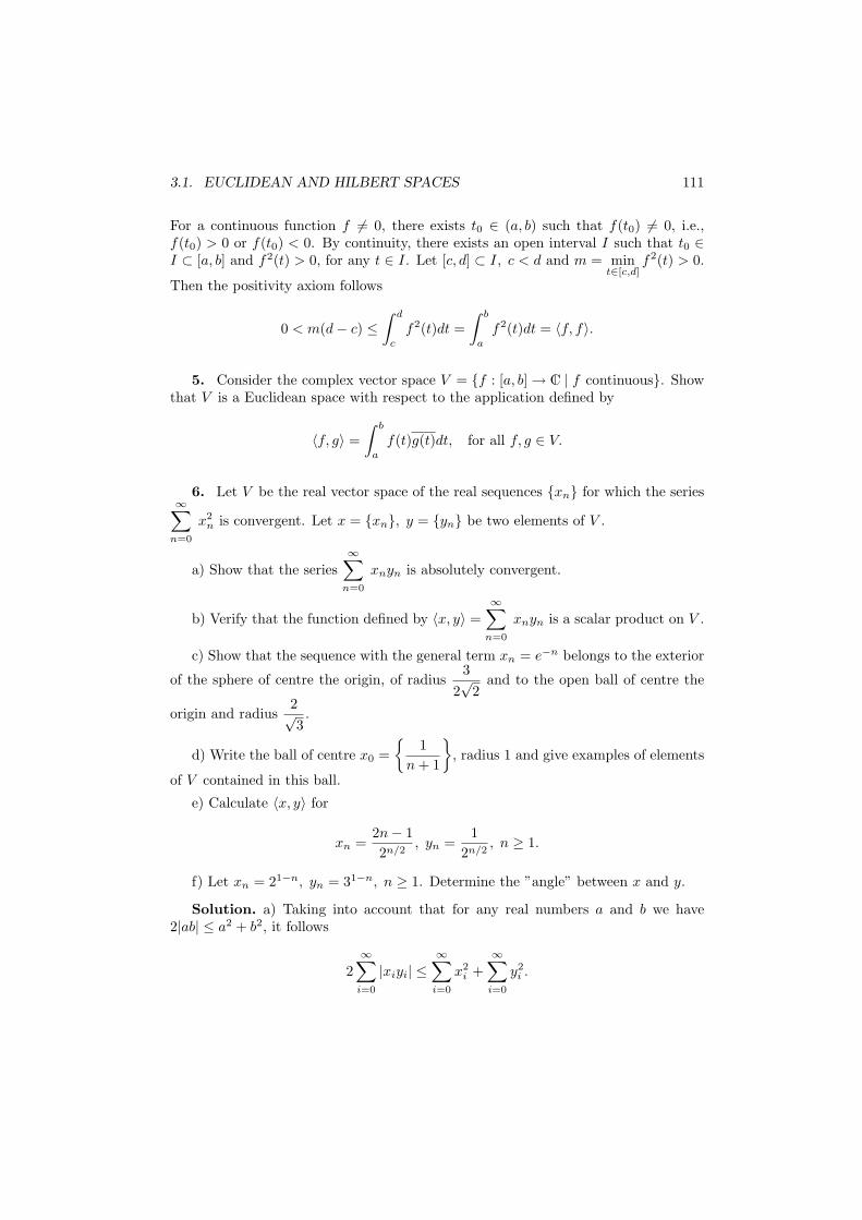
3.1. EUCLIDEAN AND HILBERT SPACES 111
For a continuous function f 6= 0, there exists t0 ∈ (a, b) such that f(t0) 6= 0, i.e.,f(t0) > 0 or f(t0) < 0. By continuity, there exists an open interval I such that t0 ∈I ⊂ [a, b] and f2(t) > 0, for any t ∈ I. Let [c, d] ⊂ I, c < d and m = min
t∈[c,d]f2(t) > 0.
Then the positivity axiom follows
0 < m(d− c) ≤∫ d
c
f2(t)dt =∫ b
a
f2(t)dt = 〈f, f〉.
5. Consider the complex vector space V = f : [a, b] → C | f continuous. Showthat V is a Euclidean space with respect to the application defined by
〈f, g〉 =∫ b
a
f(t)g(t)dt, for all f, g ∈ V.
6. Let V be the real vector space of the real sequences xn for which the series∞∑
n=0
x2n is convergent. Let x = xn, y = yn be two elements of V .
a) Show that the series∞∑
n=0
xnyn is absolutely convergent.
b) Verify that the function defined by 〈x, y〉 =∞∑
n=0
xnyn is a scalar product on V .
c) Show that the sequence with the general term xn = e−n belongs to the exterior
of the sphere of centre the origin, of radius3
2√
2and to the open ball of centre the
origin and radius2√3.
d) Write the ball of centre x0 =
1n + 1
, radius 1 and give examples of elements
of V contained in this ball.
e) Calculate 〈x, y〉 for
xn =2n− 12n/2
, yn =1
2n/2, n ≥ 1.
f) Let xn = 21−n, yn = 31−n, n ≥ 1. Determine the ”angle” between x and y.
Solution. a) Taking into account that for any real numbers a and b we have2|ab| ≤ a2 + b2, it follows
2∞∑
i=0
|xiyi| ≤∞∑
i=0
x2i +
∞∑
i=0
y2i .
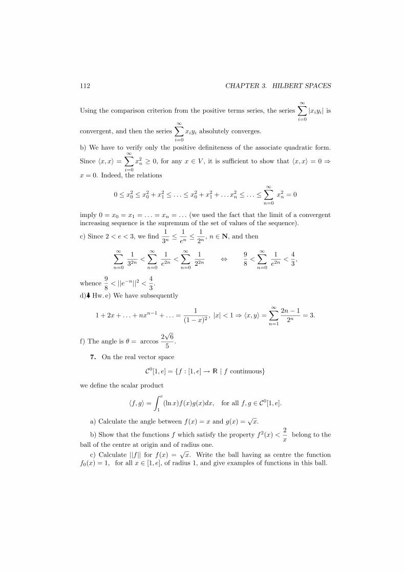
112 CHAPTER 3. HILBERT SPACES
Using the comparison criterion from the positive terms series, the series∞∑
i=0
|xiyi| is
convergent, and then the series∞∑
i=0
xiyi absolutely converges.
b) We have to verify only the positive definiteness of the associate quadratic form.
Since 〈x, x〉 =∞∑
i=0
x2n ≥ 0, for any x ∈ V , it is sufficient to show that 〈x, x〉 = 0 ⇒
x = 0. Indeed, the relations
0 ≤ x20 ≤ x2
0 + x21 ≤ . . . ≤ x2
0 + x21 + . . . x2
n ≤ . . . ≤∞∑
n=0
x2n = 0
imply 0 = x0 = x1 = . . . = xn = . . . (we used the fact that the limit of a convergentincreasing sequence is the supremum of the set of values of the sequence).
c) Since 2 < e < 3, we find13n
≤ 1en
≤ 12n
, n ∈ N, and then
∞∑n=0
132n
<
∞∑n=0
1e2n
<
∞∑n=0
122n
⇔ 98
<
∞∑n=0
1e2n
<43,
whence98
< ||e−n||2 <43.
d) Hw. e) We have subsequently
1 + 2x + . . . + nxn−1 + . . . =1
(1− x)2, |x| < 1 ⇒ 〈x, y〉 =
∞∑n=1
2n− 12n
= 3.
f) The angle is θ = arccos2√
65
.
7. On the real vector space
C0[1, e] = f : [1, e] → R | f continuouswe define the scalar product
〈f, g〉 =∫ e
1
(lnx)f(x)g(x)dx, for all f, g ∈ C0[1, e].
a) Calculate the angle between f(x) = x and g(x) =√
x.
b) Show that the functions f which satisfy the property f2(x) <2x
belong to theball of the centre at origin and of radius one.
c) Calculate ||f || for f(x) =√
x. Write the ball having as centre the functionf0(x) = 1, for all x ∈ [1, e], of radius 1, and give examples of functions in this ball.
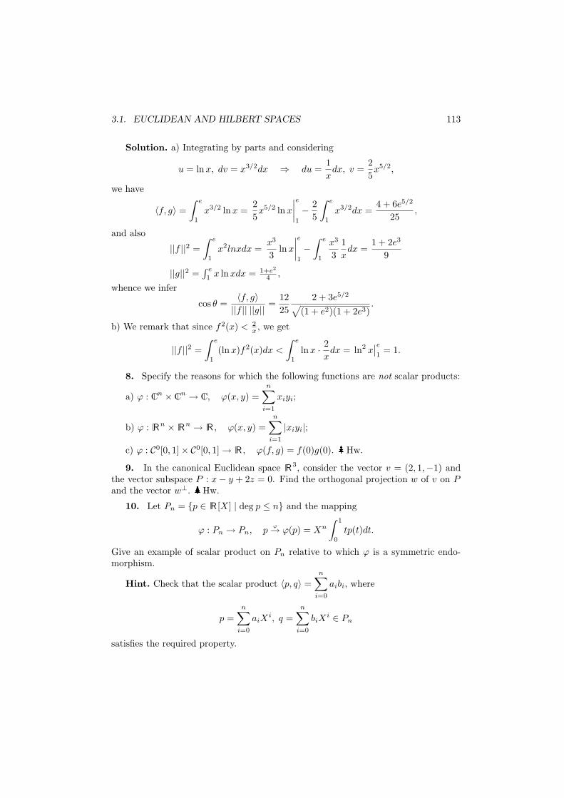
3.1. EUCLIDEAN AND HILBERT SPACES 113
Solution. a) Integrating by parts and considering
u = ln x, dv = x3/2dx ⇒ du =1x
dx, v =25x5/2,
we have
〈f, g〉 =∫ e
1
x3/2 ln x =25x5/2 ln x
∣∣∣∣e
1
− 25
∫ e
1
x3/2dx =4 + 6e5/2
25,
and also
||f ||2 =∫ e
1
x2lnxdx =x3
3ln x
∣∣∣∣e
1
−∫ e
1
x3
31x
dx =1 + 2e3
9
||g||2 =∫ e
1x ln xdx = 1+e2
4 ,
whence we infer
cos θ =〈f, g〉||f || ||g|| =
1225
2 + 3e5/2
√(1 + e2)(1 + 2e3)
.
b) We remark that since f2(x) < 2x , we get
||f ||2 =∫ e
1
(ln x)f2(x)dx <
∫ e
1
ln x · 2x
dx = ln2 x∣∣e1
= 1.
8. Specify the reasons for which the following functions are not scalar products:
a) ϕ : Cn × Cn → C, ϕ(x, y) =n∑
i=1
xiyi;
b) ϕ : Rn × Rn → R , ϕ(x, y) =n∑
i=1
|xiyi|;
c) ϕ : C0[0, 1]× C0[0, 1] → R , ϕ(f, g) = f(0)g(0). Hw.
9. In the canonical Euclidean space R3, consider the vector v = (2, 1,−1) andthe vector subspace P : x− y + 2z = 0. Find the orthogonal projection w of v on Pand the vector w⊥. Hw.
10. Let Pn = p ∈ R [X] | deg p ≤ n and the mapping
ϕ : Pn → Pn, pϕ→ ϕ(p) = Xn
∫ 1
0
tp(t)dt.
Give an example of scalar product on Pn relative to which ϕ is a symmetric endo-morphism.
Hint. Check that the scalar product 〈p, q〉 =n∑
i=0
aibi, where
p =n∑
i=0
aiXi, q =
n∑
i=0
biXi ∈ Pn
satisfies the required property.
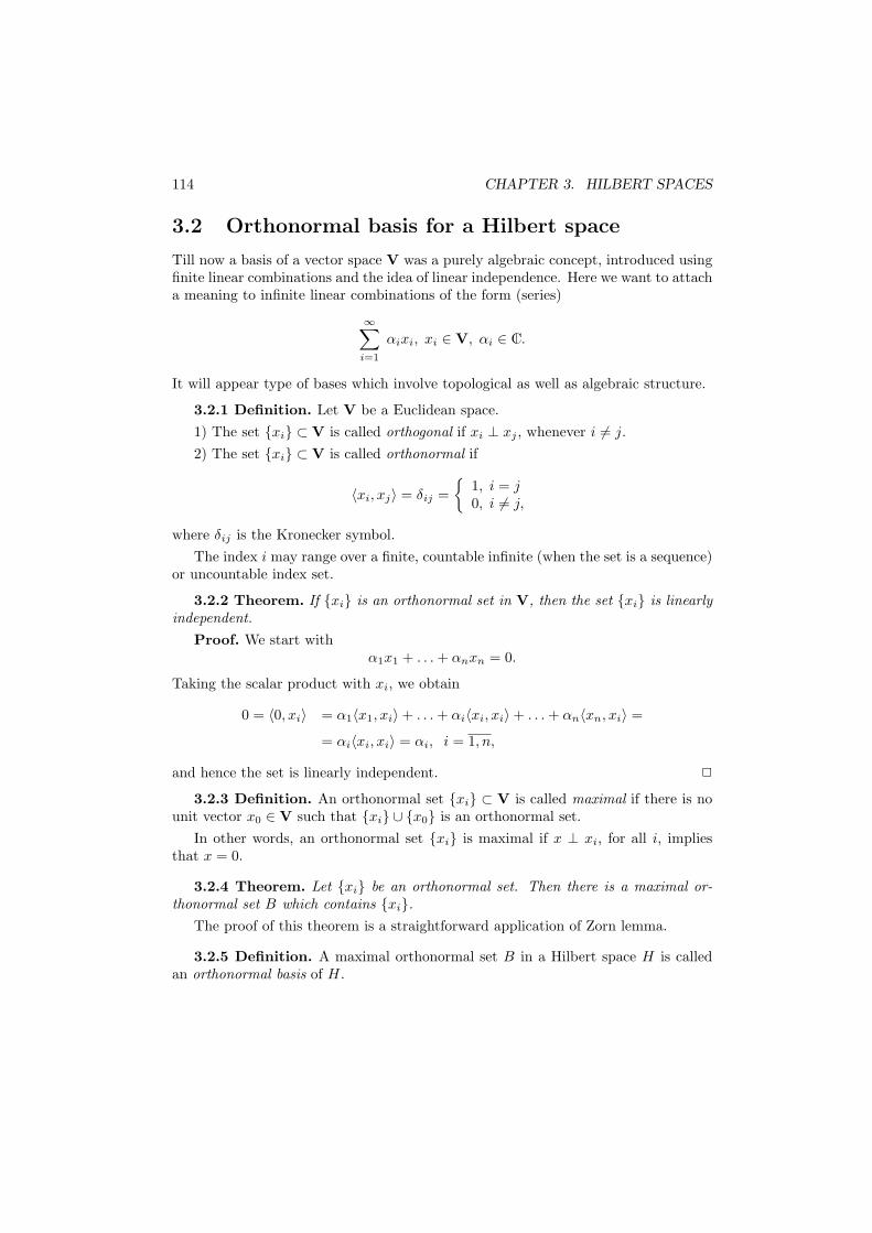
114 CHAPTER 3. HILBERT SPACES
3.2 Orthonormal basis for a Hilbert space
Till now a basis of a vector space V was a purely algebraic concept, introduced usingfinite linear combinations and the idea of linear independence. Here we want to attacha meaning to infinite linear combinations of the form (series)
∞∑
i=1
αixi, xi ∈ V, αi ∈ C.
It will appear type of bases which involve topological as well as algebraic structure.
3.2.1 Definition. Let V be a Euclidean space.1) The set xi ⊂ V is called orthogonal if xi ⊥ xj , whenever i 6= j.2) The set xi ⊂ V is called orthonormal if
〈xi, xj〉 = δij =
1, i = j0, i 6= j,
where δij is the Kronecker symbol.The index i may range over a finite, countable infinite (when the set is a sequence)
or uncountable index set.
3.2.2 Theorem. If xi is an orthonormal set in V, then the set xi is linearlyindependent.
Proof. We start withα1x1 + . . . + αnxn = 0.
Taking the scalar product with xi, we obtain
0 = 〈0, xi〉 = α1〈x1, xi〉+ . . . + αi〈xi, xi〉+ . . . + αn〈xn, xi〉 =
= αi〈xi, xi〉 = αi, i = 1, n,
and hence the set is linearly independent. 2
3.2.3 Definition. An orthonormal set xi ⊂ V is called maximal if there is nounit vector x0 ∈ V such that xi ∪ x0 is an orthonormal set.
In other words, an orthonormal set xi is maximal if x ⊥ xi, for all i, impliesthat x = 0.
3.2.4 Theorem. Let xi be an orthonormal set. Then there is a maximal or-thonormal set B which contains xi.
The proof of this theorem is a straightforward application of Zorn lemma.
3.2.5 Definition. A maximal orthonormal set B in a Hilbert space H is calledan orthonormal basis of H.
3.2. ORTHONORMAL BASIS FOR A HILBERT SPACE 115
Examples of orthonormal bases
1) I = [0, 1], H = the complex space L2(I) with the scalar product
〈f, g〉 =∫ 1
0
f(t) g(t)dt.
We claim thatΦn(t) = e2πint, n = 0,±1,±2, . . .
is an orthonormal set, i.e.,
〈Φn, Φm〉 = 0, n 6= m and ||Φn||2 = 1.
Next is possible to show that Φn is a maximal orthonormal set, i.e.,
f ⊥ Φn ⇒ f = 0.
Note. L2[a, b] = C0[a, b], where the bar means closedness.
2) The Laguerre functions form an orthonormal set for L2[0,∞). These are definedby
Φn(t) =1n!
e−t/2Ln(t), n = 0, 1, . . .
where Ln(t) are the Laguerre polynomials
Ln(t) = et dn
dtn(tne−t).
3) The Hermite functions
Φn(t) =e−t2/2
[2nn!√
π]1/2Hn(t), n = 0, 1, . . .
form an orthonormal basis for L2(−∞,∞), where
Hn(t) = (−1)net2 dn
dtn(e−t2)
are the Hermite polynomials.
4) The Legendre functions
Φn(t) =(
2n + 12
)1/2
Pn(t), n = 0, 1, . . .
form an orthonormal set for L2[−1, 1], where Pn(t) are the Legendre polynomials
Pn(t) =1
2nn!dn
dtn(t2 − 1)n.
116 CHAPTER 3. HILBERT SPACES
Note. Given any linearly independent sequence xnn∈N in a Euclidean space, itis always possible to construct an orthonormal set from it. The construction is knownas the Gram-Schmidt orthogonalization process.
3.2.6. Exercises
1. Replace the following bases with orthogonal ones:
a) v1 = (1, 1, 0), v2 = (1, 0, 1), v3 = (0, 1, 1) in R3;
b) 1, x, . . . , xn, . . . in the real vector space of all the real polynomial functionsdefined on [−1, 1].
Solution. We use the Gram-Schmidt orthogonalization method.
a) The canonical scalar product in R3 is 〈x, y〉 = x1y1 + x2y2 + x3y3. We putw1 = v1. Considering now w2 = v2 + αv1 = (1, 0, 1) + (α, α, 0) = (1 + α, α, 1),
the relation 〈w2, w1〉 = 0 is equivalent to 1 + 2α = 0, whence α = −12; it follows
w2 =(
12,−1
2, 1
).
We search similarly for w3 of the form
w3 = v3 + βw2 + γw1 = (0, 1, 1) +(
β
2,−β
2, β
)+ (γ, γ, 0) =
=(
β
2+ γ, 1− β
2+ γ, 1 + β
),
satisfying the orthogonality conditions 〈w3, w1〉 = 0 and 〈w3, w2〉 = 0, which rewrite
1 + 2γ = 03β + 1 = 0 ⇔
γ = −1
2β = − 1
3 .
Hence w3 =(−2
3,23,23
)and w1, w2, w3 is an orthogonal basis. Remark that
w1
||w1|| ,w2
||w2|| ,w3
||w3||
is an orthonormal basis.
b) We use the canonical scalar product 〈p, q〉 =∫ 1
−1
p(x)q(x)dx and the orthog-
onalization formulas. We denote pi(x) = xi, i ∈ N. Set first q0(x) = p0(x) = 1.
Computing 〈q0, q0〉 =∫ 1
−1
dx = 2, and 〈p1, q0〉 =∫ 1
−1
xdx = 0 we find
q1(x) = p1(x)− 〈p1, q0〉〈q0, q0〉 q0(x) = p1(x) = x.
3.2. ORTHONORMAL BASIS FOR A HILBERT SPACE 117
By analogy, the relations
〈p2, q0〉 =∫ 1
−1x2dx = 2
3
〈p2, q1〉 =∫ 1
−1x3dx = 0
〈q1, q1〉 =∫ 1
−1x2dx = 2
3
imply
q2(x) = p2(x)− 〈p2, q0〉〈q0, q0〉 q0(x)− 〈p2, q1〉
〈q1, q1〉 q1(x) = x2 − 13.
Similarly we find
q3(x) = x3 − 35x, q4(x) = x4 − 6
7x2 +
335
, q5(x) = x5 − 109
x3 +521
x.
By induction, it may be proved that the required polynomials qn can be computedby the formula
qn(x) =n!
(2n)!dn
dxn(x2 − 1)n, n ∈ N.
These polynomials are called the Legendre polynomials.
2. Show that equality holds in the Cauchy-Schwartz inequality |〈x, y〉| ≤ ||x|| ||y||iff the set x, y is linearly dependent.
3. Let V = L2[0, T ] be endowed with the scalar product
〈x, y〉 =∫ T
0
x(t)y(t)dt, for all x, y ∈ V
and let F be the filter mapping of V into itself defined by
(Fx)(t) =∫ t
0
e−(t−τ)x(τ)dτ, t ∈ [0, T ].
Find an input x ∈ V such that 〈x, x〉 = 1 and (Fx)(T ) is maximal.Solution. Let y(t) = et, then (Fx)(T ) = e−T 〈y, x〉. The Cauchy-Schwartz in-
equality implies|(Fx)(T )| ≤ e−T ||x|| · ||y||,
with equality when x = cy (x and y are collinear). The solution is
x(t) =
√2
e2T − 1et, t ∈ [0, T ],
and
(Fx)(T ) =
√12(1− e−2T ).
118 CHAPTER 3. HILBERT SPACES
4. Describe all possible scalar products on the complex vector space C.Show that the real vector space R2 has a scalar product which is not derived from
a complex scalar product.
5. Let 〈x, y〉 be a scalar product on the vector space V .1) Show that the mappings y → 〈x, y〉, x → 〈x, y〉 are continuous.2) Discuss the relations
⟨x,
∞∑n=1
yn
⟩=
∞∑n=1
〈x, yn〉,⟨ ∞∑
n=1
xn, y
⟩=
∞∑n=1
〈xn, y〉.
6. Let x, y be vectors in a Euclidean vector space V and assume that
||λx + (1− λ)y|| = ||x||, for all λ ∈ [0, 1].
Show that x = y.
7. Let x, y be a linearly independent set in a complex Euclidean vector spaceV . Define f : C→ R ,
f(α) = ||x− αy||, ∀α ∈ C.
Where does f take on its minimum value ?
8. Let y be a fixed vector in a Hilbert space H. Describe the operator
L : H → H, L(x) = 〈x, y〉y, for all x ∈ H.
9. Let V denote the vector subspace of L2[0, 2π] made up of all trigonometricpolynomials of the form
x(t) =n∑
k=−n
akeikt.
Let M be the subspace defined by
M =
x ∈ V
∣∣∣∣∫ 2π
0
tx(t)dt = 0
.
Let x0 in V with x0 6∈ M . Show that there is no vector y0 in M with
||x0 − y0|| = inf ||x0 − y||, y ∈ M
10. Let z = x + y, where x ⊥ y. Show that 〈z, x〉 is real.
11. Let y, z1, z2, . . . be an orthonormal set in a Hilbert space H. We constructthe linearly independent set xn n∈N
∗ by
xn =(
cos1n
)y +
(sin
1n
)zn, n ∈ N∗.
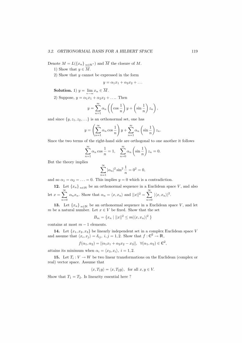
3.2. ORTHONORMAL BASIS FOR A HILBERT SPACE 119
Denote M = L(xn n∈N∗) and M the closure of M .
1) Show that y ∈ M .2) Show that y cannot be expressed in the form
y = α1x1 + α2x2 + . . .
Solution. 1) y = limn→∞
xn ∈ M .
2) Suppose, y = α1x1 + α2x2 + . . .. Then
y =∞∑
n=1
αn
((cos
1n
)y +
(sin
1n
)zn
),
and since y, z1, z2, . . . is an orthonormal set, one has
y =
( ∞∑n=1
αn cos1n
)y +
∞∑n=1
αn
(sin
1n
)zn.
Since the two terms of the right-hand side are orthogonal to one another it follows∞∑
n=1
αn cos1n
= 1,
∞∑n=0
αn
(sin
1n
)zn = 0.
But the theory implies∞∑
n=1
|αn|2 sin2 1n
= 02 = 0,
and so α1 = α2 = . . . = 0. This implies y = 0 which is a contradiction.
12. Let xn n∈N be an orthonormal sequence in a Euclidean space V , and also
let x =∞∑
n=0
αnxn. Show that αn = 〈x, xn〉 and ||x||2 =∞∑
n=0
|〈x, xn〉|2.
13. Let xn n∈N be an orthonormal sequence in a Euclidean space V , and letm be a natural number. Let x ∈ V be fixed. Show that the set
Bm = xn | ||x||2 ≤ m|〈x, xn〉|2 contains at most m− 1 elements.
14. Let x1, x2, x3 be linearly independent set in a complex Euclidean space Vand assume that 〈xi, xj〉 = δij , i, j = 1, 2. Show that f : C2 → R ,
f(α1, α2) = ||α1x1 + α2x2 − x3||, ∀(α1, α2) ∈ C2,
attains its minimum when αi = 〈x3, xi〉, i = 1, 2.
15. Let Ti : V → W be two linear transformations on the Euclidean (complex orreal) vector space. Assume that
〈x, T1y〉 = 〈x, T2y〉, for all x, y ∈ V.
Show that T1 = T2. Is linearity essential here ?
120 CHAPTER 3. HILBERT SPACES
3.3 Fourier series
Let H be a Hilbert space, and xn n∈N∗ be an orthonormal sequence. For x ∈ H,
we compute the (projections) complex numbers 〈x, xn〉, which are called the Fouriercoefficients of the vector x.
The series∞∑
n=1
〈x, xn〉xn
is called Fourier series attached to x with respect to xn.The following questions arise: a) is the series convergent ? b) is the sum of the
series equal to x ?
3.3.1 Fourier Series Theorem. Let H be a Hilbert space and xn n∈N∗ ⊂ H
be an orthonormal set. The following statements are equivalent.
1) The set xn is an orthonormal basis, i.e., it is a maximal orthonormal set.
2) (Fourier series expansion) For any x ∈ H we have x =∞∑
n=1
〈x, xn〉xn.
3) (Parseval equality) For any x, y ∈ H, one has
〈x, y〉 =∞∑
n=1
〈x, xn〉〈y, xn〉.
4) For any x ∈ H, one has
||x||2 =∞∑
n=1
|〈x, xn〉|2.
5) Let M be any vector subspace of H that contains xn n∈N∗ . Then M is dense
in H.
To prove this theorem we need three preliminary results:
• the Bessel inequality,
• discussion of the convergence of∞∑
n=1
αnxn when xn n∈N∗ is an orthonormal
sequence,
• a formula for computing orthogonal projections in terms of an orthonormalbasis.
3.3. FOURIER SERIES 121
3.3.2 (The Bessel Inequality) Lemma.If xn n∈N
∗ is an orthonormal set in a Euclidean space, then
∞∑n=1
|〈x, xn〉|2 ≤ ||x||2.
Proof. Let x1, . . . , xk ⊂ xn n∈N∗ . Then
0 ≤ ||x−k∑
i=1
〈x, xi〉xi||2 = 〈x−k∑
i=1
〈x, xi〉xi, x−k∑
j=1
〈x, xj〉xj〉 =
= 〈x, x〉 −k∑
i=1
〈x, xi〉〈xi, x〉 −k∑
j=1
〈x, xj〉〈x, xj〉+k∑
i=1
k∑
j=1
〈x, xi〉〈x, xj〉〈xi, xj〉 =
= ||x||2 −k∑
i=1
|〈x, xi〉|2,
since 〈xi, xj〉 = δij , independent of k. 2
Now let us take a careful look at the series of the form∞∑
n=1
αnxn, α ∈ C,
where xn n∈N∗ is an orthonormal sequence.
3.3.3 Lemma. Let H be a Hilbert space and xn n∈N∗ ⊂ H be an orthonormal
sequence. Then the following assertions are valid:
1)∞∑
n=1
αnxn converges iff∞∑
n=1
|αn|2 converges.
2) Assume∞∑
n=1
αnxn convergent. If
x =∞∑
n=1
αnxn =∞∑
n=1
βnxn,
then αn = βn and ||x||2 =∞∑
n=1
|αn|2.
Proof. 1) Suppose∞∑
n=1
αnxn is convergent and x =∞∑
n=1
αnxn, i.e.,
limN→∞
||x−N∑
n=1
αnxn||2 = 0.
122 CHAPTER 3. HILBERT SPACES
Since the scalar product is a continuous function, we have
〈x, xj〉 = 〈∞∑
n=1
αnxn, xj〉 =∞∑
n=1
αn〈xn, xj〉 = αj .
The Bessel inequality gives
∞∑n=1
|〈x, xn〉|2 =∞∑
n=1
|αn|2 ≤ ||x||2
and so∞∑
n=1
|αn|2 is convergent.
Next assume that∞∑
n=1
|αn|2 is convergent, and denote sn =n∑
i=1
αixi (partial
sums). It follows
||sn − sm||2 =n∑
m+1
|αi|2,
and hence sn n∈N∗ is a Cauchy sequence. The completeness of H ensures the
convergence of the sequence sn n∈N∗ .
2) Let us prove
||x||2 =∞∑
n=1
|αn|2.
For that, using the Cauchy-Schwartz inequality, we evaluate
||x||2 −N∑
n=1
|αn|2 = 〈x, x−N∑
n=1
αnxn〉+ 〈x−N∑
n=1
αnxn,
N∑n=1
αnxn〉 ≤
≤ ||x−N∑
n=1
αnxn||(||x||+ ||N∑
n=1
αnxn||) ≤
≤ 2||x|| ||x−N∑
n=1
αnxn|| → 0.
Now suppose x =∞∑
n=1
αnxn =∞∑
n=1
βnxn. This implies
0 = limN→∞
(N∑
n=1
αnxn −N∑
n=1
βnxn
)= lim
N→∞
N∑n=1
(αn − βn)xn.
Consequently
3.3. FOURIER SERIES 123
0 =∞∑
n=1
(αn − βn)xn ⇒ 02 =∞∑
n=1
|αn − βn|2 ⇒ αn = βn. 2
3.3.4 Corollary. Let H be a Hilbert space and S = xn n∈N∗ ⊂ H be an or-
thonormal sequence. The series∞∑
n=1
αnxn is convergent iff it is unconditionally con-
vergent (any rearrangement of this series is convergent).
Now we wish to show that if xn n∈N∗ ⊂ H is an orthonormal set, then the
formula
Px =∞∑
n=1
〈x, xn〉xn
defines an orthonormal projection of H onto M = L(S).For that we need the following
3.3.5 Lemma. Let B = x1, . . . , xn be a finite orthonormal set in a Hilbert spaceH and M = L(B). Then:
1) M is closed.2) The orthogonal projection of H onto M is given by
Px =n∑
i=1
〈x, xi〉xi.
Proof. 1) M is closed because is a finite dimensional subspace.2) Obviously, P : H → H is linear. Also,
Pxj =n∑
i=1
〈xj , xi〉xi = xj .
Now let x ∈ H. Then
P2x = P(
n∑
i=1
〈x, xi〉xi
)=
n∑
i=1
〈x, xi〉Pxi =n∑
i=1
〈x, xi〉xi = Px.
Consequently P is a projection.Obviously Im P ⊂ M . Conversely, for any x ∈ M we can write
x = α1x1 + . . . + αnxn.
Consequently Px = x and so Im P = M .Now we show that P is orthogonal. Let y ∈ KerP, x ∈ Im P, i.e.,
Py = 0, Px = x.
124 CHAPTER 3. HILBERT SPACES
We find
〈y, x〉 = 〈y,Px〉 = 〈y,
n∑
i=1
〈x, xi〉xi〉 =n∑
i=1
〈y, xi〉〈x, xi〉 =
=n∑
i=1
〈y, xi〉〈xi, x〉 = 〈n∑
i=1
〈y, xi〉xi, x〉 = 〈Py, x〉 = 〈0, x〉 = 0.
This concludes the proof. 2
3.3.6 Corollary (a minimum problem).Let S = x1, . . . , xn be an orthonormal set in a Hilbert space H and x ∈ H. For
any choice of complex numbers c1, . . . , cn one has
||x−n∑
i=1
〈x, xi〉xi|| ≤ ||x−n∑
i=1
cixi||.
Hint. Px =n∑
i=1
〈x, xi〉xi is the projection of x onto the subspace generated by S.
3.3.7 Lemma. Let B = xn n∈N∗ be an orthonormal sequence in H and M
be the closed vector subspace generated by B (the closure of L(B)). Then any vectorx ∈ M can be uniquely written as
x =∞∑
n=1
〈x, xn〉xn
and moreover
Px =∞∑
n=1
〈x, xn〉xn
defines the orthogonal projection of H onto M .
Proof. Let yN be a finite linear combination of vectors in B, i.e., yN =K∑
n=1
αnxn,
where both αn and K depend on N . Suppose K ≥ N . It follows
||x−K∑
n=1
〈x, xn〉xn|| ≤ ||x−K∑
n=1
αnxn|| = ||x− yN ||.
If we accept x = limN→∞
yN , then limN→∞
||x − yN || → 0. This implies x =∞∑
n=1
〈x, xn〉xn.
Then, via the Bessel inequality, we infer
||Px||2 = ||∞∑
n=1
〈x, xn〉xn||2 =∞∑
n=1
|〈x, xn〉|2 ≤ ||x||2.

3.4. CONTINUOUS LINEAR FUNCTIONALS 125
Consequently P is continuous. The orthogonality is obtained easily since continuityof the scalar product justifies the interchange of summations. 2
3.3.8 Proof of the Fourier Series Theorem
1) ⇒ 2). Hypotheses: xn n∈N∗ is a maximal orthonormal set in H, M is a
closed vectorial subspace of H generated by xn. If x ∈ M⊥, then x ⊥ xn, and sox = 0. Hence M⊥ = 0, i.e., M = H. Therefore the orthogonal projection is justthe identity
Id(x) = x =∞∑
n=1
〈x, xn〉xn.
2) ⇒ 3). For x =∞∑
n=1
〈x, xn〉xn, y =∞∑
n=1
〈y, xm〉xm we find
〈x, y〉 = 〈∞∑
n=1
〈x, xn〉xn,
∞∑n=1
〈y, xm〉xm〉 =∞∑
n=1
〈x, xn〉〈y, xn〉.
3) ⇒ 4). Obvious.4) ⇒ 1). If xn n∈N
∗ is not maximal, then there exists a unit vector x0 such thatxn n∈N
∗ ∪ x0 is an orthonormal set. But this yields the contradiction
1 = ||x0||2 =∑
|〈x0, xn〉|2 = 0.
2) ⇔ 5). The statement 5) is equivalent to ”the orthogonal projection onto M is theidentity”. Lemma 3.7 proves the equivalence with 2).
3.4 Continuous linear functionals
We want to show that every continuous linear functional on a Hilbert space has arepresentation via the scalar product.
Let V be a Euclidean vector space and y ∈ V. Define
l : V → C, l(x) = 〈x, y〉.This function is linear and
|l(x)| = |〈x, y〉| ≤ ||y|| ||x||.Consequently
||l|| = sup||x||=1
|l(x)| ≤ ||y||.
But |l(y)| = ||y|| ||y||, so ||l|| ≥ ||y||. Finally ||l|| = ||y||. Since l is bounded,automatically it is continuous.
126 CHAPTER 3. HILBERT SPACES
Consequently, a continuous linear functional l is naturally associated to each vectory: any bounded (continuous) linear functional l in a Hilbert space can be written asl(x) = 〈x, y〉, x ∈ H, y fixed in H.
3.4.1 Riesz Representation Theorem. Let H be a Hilbert space and l : H → Cbe a bounded (continuous) linear functional. Then there is one and only one vectory ∈ H such that
l(x) = 〈x, y〉, for all x ∈ H. (66)
The fixed vector y is called the representation of l.
Proof. If l = 0, then we associate y = 0 to l. Assuming that l 6= 0 we remarkthat since l is continuous, the vector subspace M = Ker l = x ∈ H|l(x) = 0 isclosed. Moreover, M 6= H, since l 6= 0. Therefore, there exist z ∈ H satisfyingz ⊥ M, ||z|| = 1.
We further show that dim M⊥ = 1 and hence z is a basis of M⊥. We note thatthe mapping l⊥ = l|M⊥ : M⊥ → C is surjective. Indeed, since l(z) 6= 0, we havedim Im l⊥ > 0. But Im l⊥ ⊂ C, hence dim Im l⊥ ≤ 1. Then dim Im ⊥l = 1 andIm l⊥ = C, l⊥ is surjective. It can be easily checked as well that l⊥ is injective, hencel⊥ is an isomorphism, whence dim M⊥ = dim C = 1.
Since z 6∈ M , one has l(z) 6= 0. First we show that l(x) = 〈x, y〉, ∀x ∈ H, fory = l(z)z. The projection theorem shows
H = M + M⊥, x = m + m⊥.
Since M⊥ = L(z), it follows that x = m + βz. Using the linearity of l and〈z, z〉 = ||z||2 = 1, we have
l(x) = l(m) + βl(z) = 0 + βl(z)〈z, z〉 = 〈m, l(z)z〉+ 〈βz, l(z)z〉 =
= 〈m + βz, l(z)z〉 = 〈x, y〉, y = l(z)z.
The vector y is unique with the property (66). Indeed, if y′ ∈ H satisfies (66) too,then
〈x, y〉 = 〈x, y′〉, for all x ∈ H,
whence 〈x, y − y′〉 = 0, for all x ∈ H. For x = y − y′ we infer 0 = 〈y − y′, y − y′〉 =||y − y′||2. It follows y = y′. 2
3.4.2. Exercise
On Rn we consider the scalar product
〈x, y〉 =n∑
i,j=1
aijxiyj .
Find a representation for l : Rn → R , when l is given by
3.5. TRIGONOMETRIC FOURIER SERIES 127
1) l(x) = x1;2) l(x) = x1 + x2;
3) l(x) =n∑
i=1
bixi.
3.5 Trigonometric Fourier series
3.5.1 We consider I = [−π, π], and the real space H = L2(I) with the scalar product
〈f, g〉 =∫ π
−π
f(t)g(t)dt.
The set
1√2π
⋃ 1√π
cos kt
∣∣∣∣ k ∈ N∗ ⋃
1√π
sin kt
∣∣∣∣ k ∈ N∗
is an orthonormal sequence. Given f ∈ H, we attach the trigonometric Fourier series
S(t) =a0
2+
∞∑
k=1
(ak cos kt + bk sin kt) ,
where
a0 =1π
∫ π
−π
f(t) dt
ak =1π
∫ π
−π
f(t) cos kt dt, k ∈ N∗
bk =1π
∫ π
−π
f(t) sin kt dt, k ∈ N∗.
(67)
Then we have the equality f(t) = S(t), for all t ∈ (−π, π).
The trigonometric Fourier series are used in the study of periodical phenomena,where appears the problem of representing a function as the sum of this kind of series.In this sense, we have two problems:
- if f is the sum of a trigonometric Fourier series, find the coefficients a0, ak, bk;
- the finding of conditions under which a function can be expanded in a trigono-metric Fourier series.
Some answers to these questions are given in §3.
3.5.2. Exercises
1. Determine the Fourier series of the function f : (−π, π) → R , f(x) = x.
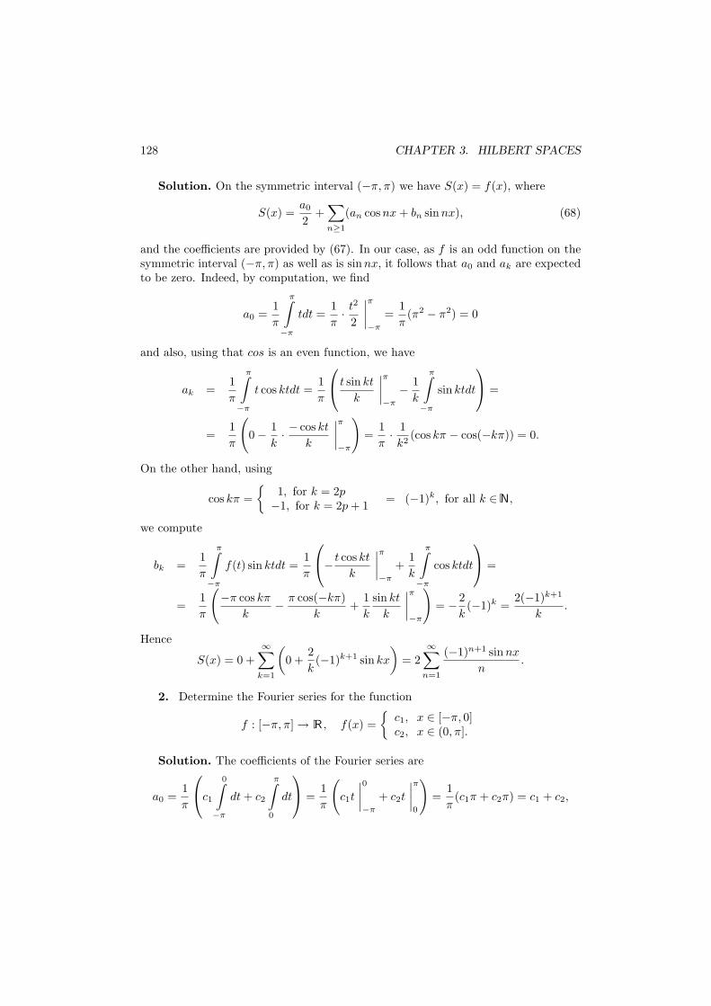
128 CHAPTER 3. HILBERT SPACES
Solution. On the symmetric interval (−π, π) we have S(x) = f(x), where
S(x) =a0
2+
∑
n≥1
(an cos nx + bn sin nx), (68)
and the coefficients are provided by (67). In our case, as f is an odd function on thesymmetric interval (−π, π) as well as is sin nx, it follows that a0 and ak are expectedto be zero. Indeed, by computation, we find
a0 =1π
π∫
−π
tdt =1π· t2
2
∣∣∣∣π
−π
=1π
(π2 − π2) = 0
and also, using that cos is an even function, we have
ak =1π
π∫
−π
t cos ktdt =1π
t sin kt
k
∣∣∣∣π
−π
− 1k
π∫
−π
sin ktdt
=
=1π
(0− 1
k· − cos kt
k
∣∣∣∣π
−π
)=
1π· 1k2
(cos kπ − cos(−kπ)) = 0.
On the other hand, using
cos kπ =
1, for k = 2p−1, for k = 2p + 1 = (−1)k, for all k ∈ N,
we compute
bk =1π
π∫
−π
f(t) sin ktdt =1π
− t cos kt
k
∣∣∣∣π
−π
+1k
π∫
−π
cos ktdt
=
=1π
(−π cos kπ
k− π cos(−kπ)
k+
1k
sin kt
k
∣∣∣∣π
−π
)= −2
k(−1)k =
2(−1)k+1
k.
Hence
S(x) = 0 +∞∑
k=1
(0 +
2k
(−1)k+1 sin kx
)= 2
∞∑n=1
(−1)n+1 sin nx
n.
2. Determine the Fourier series for the function
f : [−π, π] → R , f(x) =
c1, x ∈ [−π, 0]c2, x ∈ (0, π].
Solution. The coefficients of the Fourier series are
a0 =1π
c1
0∫
−π
dt + c2
π∫
0
dt
=
1π
(c1t
∣∣∣∣0
−π
+ c2t
∣∣∣∣π
0
)=
1π
(c1π + c2π) = c1 + c2,
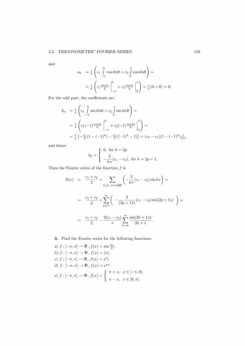
3.5. TRIGONOMETRIC FOURIER SERIES 129
and
ak = 1π
(c1
0∫−π
cos ktdt + c2
π∫0
cos ktdt
)=
= 1π
(c1
sin ktk
∣∣∣∣0
−π
+ c2sin kt
k
∣∣∣∣π
0
)= 1
π (0 + 0) = 0;
For the odd part, the coefficients are
bk = 1π
(c1
0∫−π
sin ktdt + c2
π∫0
sin ktdt
)=
= 1π
(c1(−1) cos kt
k
∣∣∣∣0
−π
+ c2(−1) cos ktk
∣∣∣∣π
0
)=
= 1π
(− c1k (1− (−1)k)− c2
k ((−1)k − 1))
= (c2 − c1)(1− (−1)k) 1kπ ,
and hence
bk =
0, for k = 2p
− 2kπ
(c1 − c2), for k = 2p + 1.
Then the Fourier series of the function f is
S(x) =c1 + c2
2+
∑
k≥1; k=odd
(− 2
kπ(c1 − c2) sin kx
)=
=c1 + c2
2+
∞∑
p≥0
(− 2
(2p + 1)π(c1 − c2) sin(2p + 1)x
)=
=c1 + c2
2− 2(c1 − c2)
π
∞∑
k=0
sin(2k + 1)x2k + 1
.
3. Find the Fourier series for the following functions:
a) f : [−π, π] → R , f(x) = sin 3x2 ;
b) f : [−π, π] → R , f(x) = |x|;c) f : [−π, π] → R , f(x) = x2;
d) f : [−π, π] → R , f(x) = eax.
e) f : [−π, π] → R , f(x) =
π + x, x ∈ [−π, 0)
π − x, x ∈ [0, π].
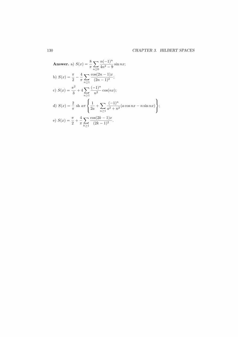
130 CHAPTER 3. HILBERT SPACES
Answer. a) S(x) =8π
∑
n≥0
n(−1)n
4n2 − 9sin nx;
b) S(x) =π
2− 4
π
∑
n≥1
cos(2n− 1)x(2n− 1)2
;
c) S(x) =π2
3+ 4
∑
n≥1
(−1)n
n2cos(nx);
d) S(x) =2π
sh aπ
12a
+∑
n≥1
(−1)n
a2 + n2(a cosnx− n sin nx)
;
e) S(x) =π
2+
4π
∑
k≥1
cos(2k − 1)x(2k − 1)2
.
Chapter 4
Numerical Methods in LinearAlgebra
4.1 The norm of a matrix
Consider the n-dimensional real vector space Rn.
4.1.1 Definition. We call norm in Rn a mapping || · || : x ∈ Rn → ||x|| ∈ R+,satisfying the following conditions
1. positivity: ||x|| ≥ 0, for all x ∈ V and
||x|| = 0 ⇔ x = 0;
2. homogeneity: ||αx|| = |α|||x||, for all x ∈ V;
3. the triangle inequality: ||x + y|| ≤ ||x||+ ||y||, for all x, y ∈ V.Examples. The so-called Lp - norms on Rn, for p ∈ [1,∞), which are provided
by
||x||p =
(n∑
i=1
|xi|p)1/p
, for all x = t(x1, . . . , xn) ∈ Rn,
satisfy the conditions 1-3 from above. As particular cases, we have:
a) for p = 1, we get ||x||1 = |x1|+ |x2|+ . . . + |xn|, (the sky-scrapper norm);
b) for p = 2, we have ||x||2 =√
x21 + . . . + x2
n =√〈x, x〉, (the Euclidean norm);
c) for p = ∞, we find ||x||∞ = maxi∈1,n
|xi|, (the ”max” norm).
Remark that, for p = 2, we have 〈x, y〉 = txy, and the Cauchy-Schwartz inequalityholds true
|〈x, y〉| ≤ ||x|| · ||y||, for all x, y ∈ Rn.
131
132 CHAPTER 4. NUMERICAL METHODS IN LINEAR ALGEBRA
4.1.2 Theorem. Let || · ||♦, || · ||♣ be two norms on Rn. Then there exist a, b > 0such that
a|| · ||♦ ≤ || · ||♣ ≤ b|| · ||♦.
Practically, the theorem states that any two norms on Rn are equivalent.
Remark. The theorem is no longer valid for infinite dimensional vector spaces.Let A = (aij)i=1,m,j=1,n ∈ Mm×n( R). The matrix A defines uniquely a linear
operator
LA : Rn → Rm, LA(x) = Ax, for all x = t(x1, . . . , xn) ∈ Rn.
Let Rn and Rm be endowed with the norms || · ||♦ and || · ||♣, respectively.
4.1.3 Theorem. The real function || · || : Mm×n( R) → R+ given by
||A|| = sup||x||♦=1
||LA(x)||♣.
is a norm on the mn - dimensional real vector space Mm×n( R) of matrices.
Proof. The positivity. Since ||LA(x)||♣ ≥ 0, for all x ∈ Rn, it follows ||A|| ≥ 0.We have then
||A|| = 0 ⇒ ||LA(x)||♣ = 0, for all x ∈ Rn,
whenceLA(x) = 0, for all x ∈ Rn ⇒ LA = 0 ⇒ A = 0.
If A = 0, obviously LA = 0 ⇒ LA(x) = 0, for all x ∈ Rn ⇒ ||A|| = 0. The other twoproperties of the norm are left as exercises. 2
Remarks. 1o. If m = n and || · ||1 = || · ||2 = || · ||, then we have
||AB|| ≤ ||A|| · ||B||, for all A,B ∈ Mn(R).
2o. For || · ||1 and || · ||2, we can consider any of the norms described in 1.1. In thecase presented above, if || · ||1 = || · ||2 = || · ||•, then we denote the norm of the matrixA simply by ||A||•.
4.1.4 Theorem. If Rm and Rn are endowed with Lp - norms, p ∈ 1, 2,∞,then the following equalities hold true
||A||1 def= sup||x||1=1
||Ax||1 = maxj=1,n
m∑i=1
|aij |
||A||∞ def= sup||x||∞=1
||Ax||∞ = maxi=1,m
n∑j=1
|aij |
||A||2 def= sup||x||2=1
||Ax||2 =√
max |λ| | λ ∈ σ(tAA) .
4.1. THE NORM OF A MATRIX 133
Proof. Denote ||A||♦ = maxj=1,n
m∑i=1
|aij |. Rewriting in coordinates the equality y =
Ax, for all x = t(x1, . . . , xn) ∈ Rn we have yi =n∑
j=1
aijxj , i = 1,m. Then
||Ax||1 = ||y||1 =m∑
i=1
|yi| =m∑
i=1
∣∣∣∣∣n∑
j=1
aijxj
∣∣∣∣∣ ≤
≤m∑
i=1
n∑j=1
|aij ||xj | =n∑
j=1
|xj |(
n∑i=1
|aij |)≤
≤n∑
j=1
|xj |(
maxj=1,n
n∑i=1
|aij |)
=n∑
j=1
|xj |||A||♦ = ||A||♦||x||1.
Then
||Ax||1 ≤ ||A||♦||x||1 ⇒ ||A(
1||x||x
)||1 ≤ ||A||♦ ⇒ sup
||v||1=1
||Av||1 ≤ ||A||♦, (69)
whence ||A||1 ≤ ||A||♦.
Denoting ek = t(0, . . . , 1, . . . , 0)(1 in the k-th pos.)
and Aek = t(ak1, . . . , akn), it follows that
||Aek||1 =m∑
i=1
|aik|, k = 1, n.
Hence, if maxj=1,n
m∑i=1
|aij | is attended on index j = k then, using the relation above, we
find
||A||♦ = maxj=1,n
m∑
i=1
|aij | = ||Aek||1,
and since ||ek||1 = 1, we have
||A||1 = sup||x||1=1
||Ax||1 ≥ ||Aek|| = ||A||♦ ⇒ ||A||1 ≥ ||A||♦. (70)
From (69), (70), the two norms coincide, i.e., ||A||1 ≡ ||A||♦.For ||A||∞ the proof is similar. For ||A||2, remark that
||Ax||2 =√
tx tAAx =√
txBx,
where we denote B = tAA. But B is symmetrical, hence it has real eigenvaluesσ(A) = λ1, . . . , λn, and moreover, these are nonnegative; for |λ1| ≤ |λ2| ≤ . . . ≤|λn|, we have
|λ1| txx ≤ |txBx| ≤ |λn| txx, for all x ∈ Rn.
134 CHAPTER 4. NUMERICAL METHODS IN LINEAR ALGEBRA
Then we obtain
|λ1| ≤ |txBx|||x||22
≤ |λn|, for all x ∈ Rn.
Denoting v = 1||x||2 x, and hence ||v||2 = 1, we find
||Av||2 =||Ax||2||x||2 =
√txBxtxx
∈[√
|λ1|,√|λn|
],
so that
||A||2 = sup||v||=1
||Av||2 ≤ |λn| ⇒ ||A||2 ≤√
max|λ| | λ ∈ σ (tAA).
The converse inequality holds also true. 2
Corollary. If A = tA ∈ Mn( R), then ||A||2 = max |λi| | λi ∈ σ(A) .Proof. In this case the eigenvalues of B =t AA are exactly the squares of those of
the matrix A, whence the result. 2
4.1.5 Definition. Let A ∈ Mn( R), det A 6= 0. The number
k(A) = ||A|| · ||A−1||
is called the conditioning number of the matrix A relative to the particular norm usedin the definition.
Remark. Consider the norm || · ||2 on
GLn( R) = A | A ∈ Mn(R), det A 6= 0.
Since1 = ||I||2 = ||AA−1||2 ≤ ||A||2 · ||A−1||2 = k(A),
we getk(A) ≥ 1, for all A ∈ GLn(R).
4.1.6. Exercises
1. a) Compute ||v||p, for v = t(1, 0,−2), and p ∈ 1, 2,∞.b) Compute ||A||p for A =
(1 0−1 2
), and p ∈ 1, 2,∞.
Solution. a) By straightforward computation, we obtain
||v||1 = |1|+ |0|+ | − 2| = 3
||v||2 =√
1 + 0 + 4 =√
5
||v||∞ = max|1|, |0|, | − 2| = 2.
4.1. THE NORM OF A MATRIX 135
b) Using the theorem which characterizes the p–norms of matrices A ∈ Mm×n(R),we infer
||A||1 = maxj=1,n
m∑i=1
|aij | = max|1|+ | − 1|, |0|+ |2| = 2
||A||2 = maxλ∈σ(tA A)
√|λ| = max
λ∈3±√5
√|λ| =
√3 +
√5
||A||∞ = maxi=1,m
n∑j=1
|aij | = max|1|+ | − 0|, | − 1|+ |2| = 3.
The last norm was obtained following the computations
tAA =(
1 −10 2
)·(
1 0−1 2
)=
(2 −2−2 4
),
whence
PtAA(λ) =∣∣∣∣
2− λ −2−2 4− λ
∣∣∣∣ = λ2 − 6λ + 4 = 0 ⇒ λ1,2 = 3±√
5.
2. a) Check that the spectral radius ρ(A) = max |λ| | λ ∈ σ(A) ⊂ C of the
matrix A =(
1 0−1 2
)is less or equal than any of the norms of A of the previous
problem.b) Find the conditioning number of A with respect to the three considered norms.
c) Compute ρ(B) and ||B||2, for B =(
1 11 2
).
Solution. a) In this case σ(A) = 1, 2, whence
ρ(A) = maxλ∈σ(A)
|λ| = 2.
We have tA A =(
2 −2−2 4
)and the three norms of A are
||A||1 = 2, ||A||∞ = 3, ||A||2 =√
3 +√
5;
remark that all are greater or equal to ρ(A) = 2.
b) The inverse is A−1 =(
1 012
12
), t(A−1)A−1 =
(5/4 1/41/4 1/4
), and the norms of
A−1 are
||A−1||1 =32, ||A−1||∞ = 1, ||A−1||2 =
√3 +
√5
2.
Then the corresponding conditioning numbers are
k1(A) = 3, k∞(A) = 3, k2(A) =3 +
√5
2.
136 CHAPTER 4. NUMERICAL METHODS IN LINEAR ALGEBRA
c) The characteristic polynomial of B is PB(λ) = λ2 − 3λ + 1, whence its roots
are λ1,2 = (3 ± √5)/2 and hence ρ(B) = (3 +√
5)/2. As well, tBB =(
2 33 5
),
σ(tBB) = (7± 3√
5)/2 whence
||B||2 = maxλ∈σ(tBB)
√|λ| =
√(7 + 3
√5)/2.
We note that ||B||2 = ρ(B), since B = tB.
4.2 The inverse of a matrix
Let A ∈ Mn( R). We try to relate the spectrum of A, σ(A) = λ1, . . . , λn ⊂ C tothe norms of the matrix A.
4.2.1 Definition. The real positive number ρ(A) = maxi=1,n
|λi| is called the
spectral radius of the matrix A.
If u ∈ Rn\0 is an eigenvector associated to λ ∈ σ(A), then, considering theassociated unit vector v = 1
||u||u, (||v|| = 1), we find
Au = λu ⇒ ||Au|| = |λ| · ||u|| ⇒ ||Au||||u|| = |λ| ⇒ |λ| = ||Av||.
Then |λ| ≤ sup||w||=1
||Aw|| = ||A||. So that for all λ ∈ σ(A), we have |λ| ≤ ||A||, whence
maxλi∈σ(A)
| λi |≤ ||A||, and thus
ρ(A) ≤ ||A||. (71)
4.2.2 Theorem. a) For all ε > 0, there exists a norm || · || : Mn( R) → R+, suchthat
||A|| ≤ ρ(A) + ε, for all A ∈ Mn( R).
b) Let A ∈ Mn(R). We have limk→∞
Ak = 0n×n if and only if ρ(A) < 1.
Proof. b) We prove first the direct implication by reductio ad absurdum. Letlim
k→∞Ak = 0 and let λ ∈ σ(A) be an eigenvalue such that |λ| ≥ 1, and let x ∈ Rn\0
be a corresponding eigenvector, assumed unit vector. But Akx = λkx, for all k ∈ N∗,whence
limk→∞
||Akx|| = limk→∞
||λkx|| = limk→∞
|λ|k ≥ 1,
since |λ| ≥ 1. So that
||Ak|| = sup||v||=1
||Akv|| ≥ ||Akx|| ≥ 1,
4.2. THE INVERSE OF A MATRIX 137
Thus we have limk→∞
||Ak|| 6= 0, so limk→∞
Ak 6= 0n×n, which contradicts the initial asser-tion.
The converse implication. If ρ(A) < 1, according to a) there exists a norm || · ||♦,such that ||A||♦ < 1. Then
0 ≤ ||Ak||♦ ≤ ||A||♦k−→k→∞
0,
and it follows that limk→∞
||Ak||♦ = 0, whence limk→∞
Ak = 0n×n. 2
4.2.3 Theorem. Let B ∈ Mn(R) be a matrix such that ρ(B) < 1. Then I − Bis invertible, and
(I −B)−1 = limk→∞
k∑
i=0
Bi =∞∑
i=0
Bi,
where we denoted B0 = In.
Proof. If ρ(B) < 1, then (I −B) has no vanishing eigenvalue, therefore
det (I −B) = λ1 . . . λn 6= 0,
i.e., is non degenerate, and hence invertible. Using the equalities
BmBn = BnBm = Bm+n,
we find(I −B)(I + B + . . . + Bk−1) = I −Bk,
whence for k →∞ we obtain the result,
(I −B) limk→∞
k−1∑
i=0
Bi = I − limk→∞
Bk.
Corollary. If ||B|| < 1, then the matrix I −B is invertible, and we have
||(I −B)−1|| ≤∞∑
i=0
||B||i.
Proof. The invertibility follows from ρ(B) ≤ ||B|| < 1 and from the theoremabove. Also, using the relation
||AB|| ≤ ||A|| · ||B||,we obtain
||(I −B)−1|| ≤∞∑
i=1
||Bi|| ≤∞∑
i=1
||B||i =1
1− ||B|| . 2
138 CHAPTER 4. NUMERICAL METHODS IN LINEAR ALGEBRA
4.2.4 Definitions. a) Let A be an invertible matrix A ∈ Gl(n, R) and let b ∈ Rn.We consider the linear system
Ax = b, (72)
in the unknown x ∈ Rn, and call x = A−1b the exact solution of the system (72).b) Let ε ∈ Mn(R) be a matrix called rounding error, assumed to satisfy ||ε|| ¿
||A||. Consider the linear attached system
(A + ε)x = b; (73)
if the matrix A + ε is invertible, then we call x = (A + ε)−1b the approximatesolution of the initial system. In this case, the quantity
e =||x− x||||x|| ,
where x is the solution of the initial equation, is called the relative error.
Remark. Denote u = x− x (and hence x = x + u), and assume that ||u|| < ||x||.Then the attached system (73) becomes: (A + ε)(x + u) = b. Using the relationAx = b fulfilled by x, the approximation εu ' 0 which holds for ε, u small, and thefact that A is invertible, we obtain
Au + εx = 0 ⇒ u = −A−1εx,
and hence ||u|| ≤ ||A−1|| · ||ε|| · ||x||. The relative error becomes
e =||x− x||||x|| =
||u||||x|| ≤
||A−1|| · ||ε|| · ||x||||x|| = ||A|| · ||A−1|| ||ε||||A|| .
The quantityk(A) = ||A|| · ||A−1||
was called conditioning number of the matrix A, with respect to the norm || · ||.For k(A) having large values, the relative error increases and the computational
methods give inaccurate results.
Example. Compute the exact solution, the approximate solution and the condi-tioning number of the following linear system, for the rounding error ε
2a + 1b = 3−2a + 3b = 1 , ε =
(0.5 00 0.1
).
Solution. The given linear system rewrites
Ax = b ⇔(
2 1−2 3
)(ab
)=
(31
),
4.3. TRIANGULARIZATION OF A MATRIX 139
and has the exact solution x = t(a, b) = t(1, 1). The altered system
(A + ε)x = b ⇔
2.5a + 1b = 3−2a + 3.1b = 1
has the solution x =(
166195
,3439
). Then x is close to x iff the number k(A) is sufficiently
small.Hw.Compute k(A) = ||A|| · ||A−1|| for || · ||2.
4.3 Triangularization of a matrix
The idea of this section is to decompose a given matrix as a product between a lower-triangular and an upper-triangular matrix. Then the linear systems whose matrix ofcoefficients is the decomposed matrix become equivalent to triangular linear systemswhich can be solved in straightforward manner.
4.3.1 Definitions. a) A quadratic matrix in which all elements are zero above/belowthe diagonal is called lower/upper triangular matrix.
b) Let A ∈ Mn(R), A = (aij)1,n×1,n. Then the matrix blocks
A[k] ∈ Mk(R), A[k] = (aij)i,j=1,k, k = 1, n
are called principal submatrices of A.
Example. The following matrix is upper triangular
1 2 30 2 10 0 1
.
Theorem. If det (A[k]) 6= 0, for all k = 1, n− 1, then there exists a non-singular lower triangular matrix M ∈ Mn( R), such that MA = U , where U isupper-triangular. Thus, for L = M−1, the matrix A decomposes as A = LU (theLU decomposition of A).
Proof. We search for M of the form M = Mn−1 . . . M1, where Mk = In−mktek,
withmk = t(0, . . . , 0, µk+1,k, . . . , µn,k), ek = t (0, . . . , 0, 1, 0, . . . , 0)︸ ︷︷ ︸
1 in the k-th position
.
We remark that:1) M−1
k = In + mktek, for all k = 1, n− 1.
2) If x = t(ζ1, . . . , ζk, ζk+1, .., ζn) is the k−th column of the matrix
Mk−1Mk−2 . . . M1A
(or A, in case that k = 1), and if tekx ≡ ζk 6= 0 (satisfied due to the requirementsimposed on A), then there exists an upper-triangular matrix Mk such that in the
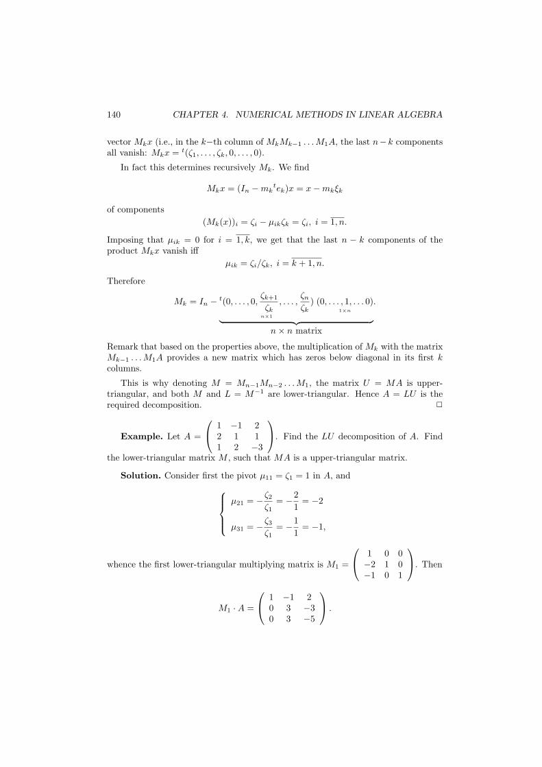
140 CHAPTER 4. NUMERICAL METHODS IN LINEAR ALGEBRA
vector Mkx (i.e., in the k−th column of MkMk−1 . . . M1A, the last n−k componentsall vanish: Mkx = t(ζ1, . . . , ζk, 0, . . . , 0).
In fact this determines recursively Mk. We find
Mkx = (In −mktek)x = x−mkξk
of components(Mk(x))i = ζi − µikζk = ζi, i = 1, n.
Imposing that µik = 0 for i = 1, k, we get that the last n − k components of theproduct Mkx vanish iff
µik = ζi/ζk, i = k + 1, n.
Therefore
Mk = In − t(0, . . . , 0,ζk+1
ζk, . . . ,
ζn
ζk)
n×1
(0, . . . , 1, . . . 0)1×n
︸ ︷︷ ︸n× n matrix
.
Remark that based on the properties above, the multiplication of Mk with the matrixMk−1 . . .M1A provides a new matrix which has zeros below diagonal in its first kcolumns.
This is why denoting M = Mn−1Mn−2 . . . M1, the matrix U = MA is upper-triangular, and both M and L = M−1 are lower-triangular. Hence A = LU is therequired decomposition. 2
Example. Let A =
1 −1 22 1 11 2 −3
. Find the LU decomposition of A. Find
the lower-triangular matrix M , such that MA is a upper-triangular matrix.
Solution. Consider first the pivot µ11 = ζ1 = 1 in A, and
µ21 = −ζ2
ζ1= −2
1= −2
µ31 = −ζ3
ζ1= −1
1= −1,
whence the first lower-triangular multiplying matrix is M1 =
1 0 0−2 1 0−1 0 1
. Then
M1 ·A =
1 −1 20 3 −30 3 −5
.
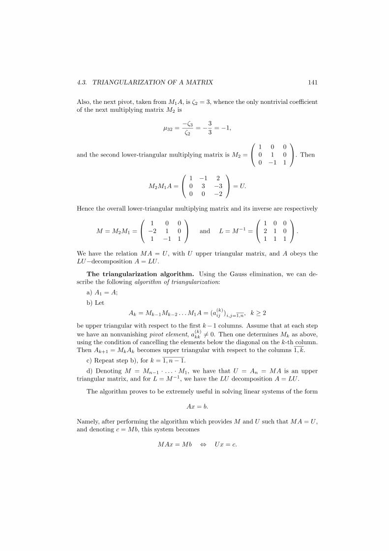
4.3. TRIANGULARIZATION OF A MATRIX 141
Also, the next pivot, taken from M1A, is ζ2 = 3, whence the only nontrivial coefficientof the next multiplying matrix M2 is
µ32 =−ζ3
ζ2= −3
3= −1,
and the second lower-triangular multiplying matrix is M2 =
1 0 00 1 00 −1 1
. Then
M2M1A =
1 −1 20 3 −30 0 −2
= U.
Hence the overall lower-triangular multiplying matrix and its inverse are respectively
M = M2M1 =
1 0 0−2 1 01 −1 1
and L = M−1 =
1 0 02 1 01 1 1
.
We have the relation MA = U , with U upper triangular matrix, and A obeys theLU−decomposition A = LU .
The triangularization algorithm. Using the Gauss elimination, we can de-scribe the following algorithm of triangularization:
a) A1 = A;
b) Let
Ak = Mk−1Mk−2 . . .M1A = (a(k)ij )i,j=1,n, k ≥ 2
be upper triangular with respect to the first k−1 columns. Assume that at each stepwe have an nonvanishing pivot element, a
(k)kk 6= 0. Then one determines Mk as above,
using the condition of cancelling the elements below the diagonal on the k-th column.Then Ak+1 = MkAk becomes upper triangular with respect to the columns 1, k.
c) Repeat step b), for k = 1, n− 1.
d) Denoting M = Mn−1 · . . . · M1, we have that U = An = MA is an uppertriangular matrix, and for L = M−1, we have the LU decomposition A = LU .
The algorithm proves to be extremely useful in solving linear systems of the form
Ax = b.
Namely, after performing the algorithm which provides M and U such that MA = U ,and denoting c = Mb, this system becomes
MAx = Mb ⇔ Ux = c.
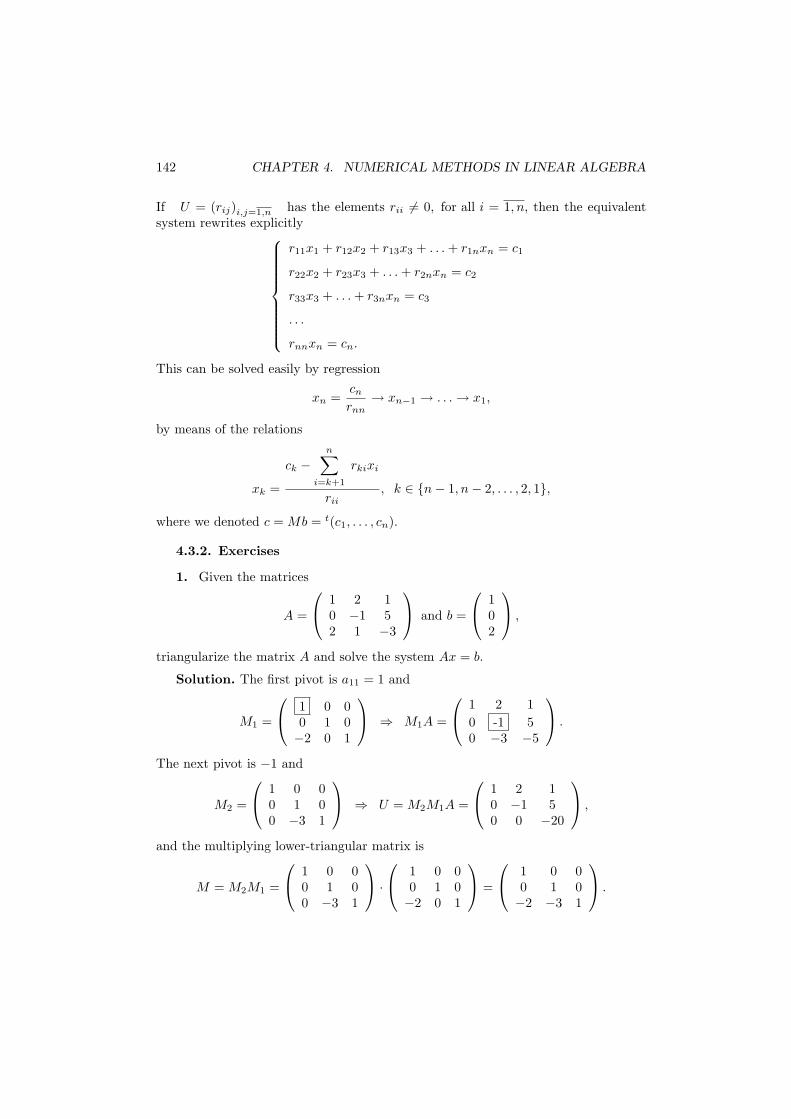
142 CHAPTER 4. NUMERICAL METHODS IN LINEAR ALGEBRA
If U = (rij)i,j=1,n has the elements rii 6= 0, for all i = 1, n, then the equivalentsystem rewrites explicitly
r11x1 + r12x2 + r13x3 + . . . + r1nxn = c1
r22x2 + r23x3 + . . . + r2nxn = c2
r33x3 + . . . + r3nxn = c3
. . .
rnnxn = cn.
This can be solved easily by regression
xn =cn
rnn→ xn−1 → . . . → x1,
by means of the relations
xk =
ck −n∑
i=k+1
rkixi
rii, k ∈ n− 1, n− 2, . . . , 2, 1,
where we denoted c = Mb = t(c1, . . . , cn).
4.3.2. Exercises
1. Given the matrices
A =
1 2 10 −1 52 1 −3
and b =
102
,
triangularize the matrix A and solve the system Ax = b.
Solution. The first pivot is a11 = 1 and
M1 =
1 0 00 1 0−2 0 1
⇒ M1A =
1 2 10 -1 50 −3 −5
.
The next pivot is −1 and
M2 =
1 0 00 1 00 −3 1
⇒ U = M2M1A =
1 2 10 −1 50 0 −20
,
and the multiplying lower-triangular matrix is
M = M2M1 =
1 0 00 1 00 −3 1
·
1 0 00 1 0−2 0 1
=
1 0 00 1 0−2 −3 1
.
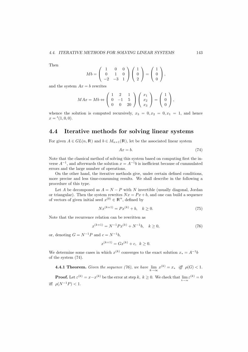
4.4. ITERATIVE METHODS FOR SOLVING LINEAR SYSTEMS 143
Then
Mb =
1 0 00 1 0−2 −3 1
102
=
100
,
and the system Ax = b rewrites
MAx = Mb ⇔
1 2 10 −1 50 0 20
x1
x2
x3
=
100
,
whence the solution is computed recursively, x3 = 0, x2 = 0, x1 = 1, and hencex = t(1, 0, 0).
4.4 Iterative methods for solving linear systems
For given A ∈ GL(n, R) and b ∈ Mn×1(R), let be the associated linear system
Ax = b. (74)
Note that the classical method of solving this system based on computing first the in-verse A−1, and afterwards the solution x = A−1b is inefficient because of cummulatederrors and the large number of operations.
On the other hand, the iterative methods give, under certain defined conditions,more precise and less time-consuming results. We shall describe in the following aprocedure of this type.
Let A be decomposed as A = N − P with N invertible (usually diagonal, Jordanor triangular). Then the system rewrites Nx = Px + b, and one can build a sequenceof vectors of given initial seed x(0) ∈ Rn, defined by
Nx(k+1) = Px(k) + b, k ≥ 0. (75)
Note that the recurrence relation can be rewritten as
x(k+1) = N−1Px(k) + N−1b, k ≥ 0, (76)
or, denoting G = N−1P and c = N−1b,
x(k+1) = Gx(k) + c, k ≥ 0.
We determine some cases in which x(k) converges to the exact solution x∗ = A−1bof the system (74).
4.4.1 Theorem. Given the sequence (76), we have limk→∞
x(k) = x∗ iff ρ(G) < 1.
Proof. Let ε(k) = x−x(k) be the error at step k, k ≥ 0. We check that limk→∞
ε(k) = 0
iff ρ(N−1P ) < 1.
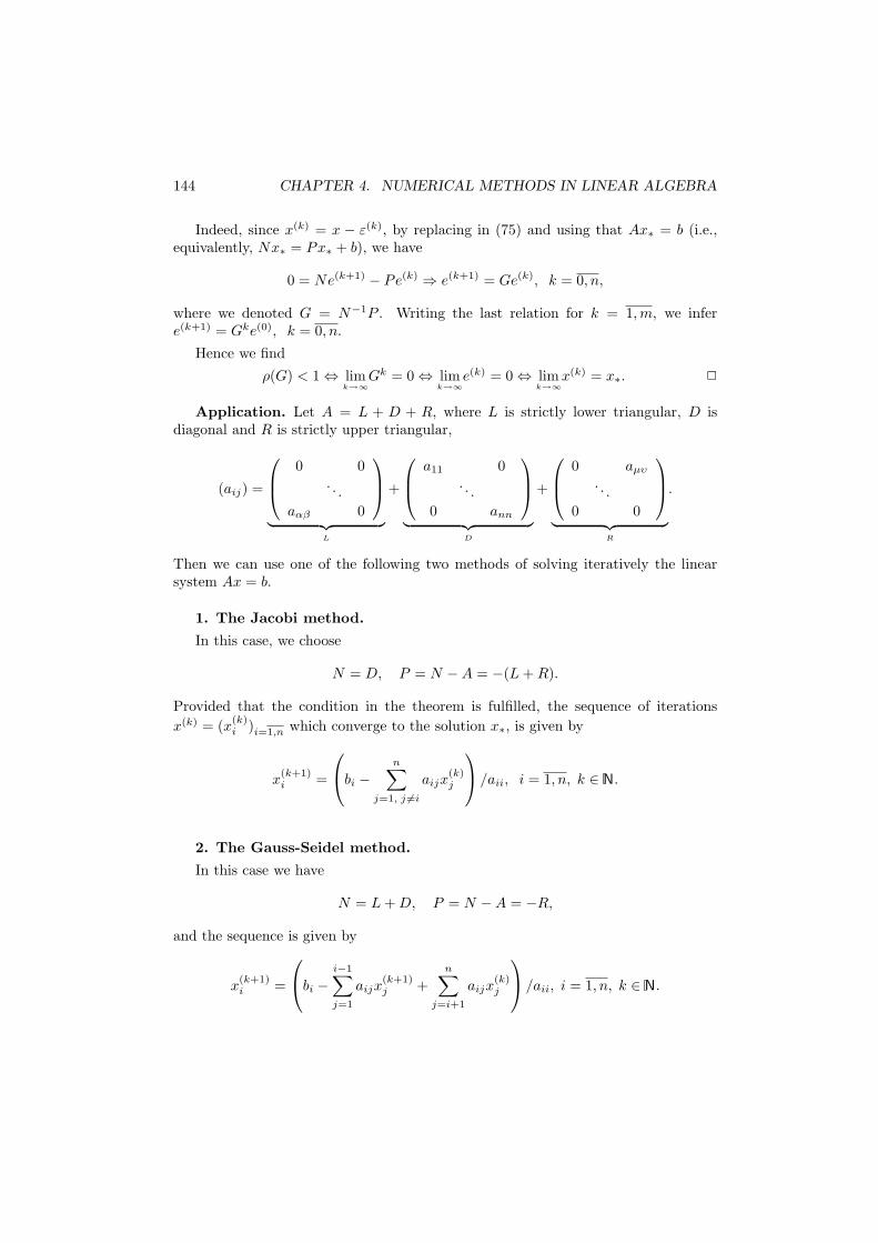
144 CHAPTER 4. NUMERICAL METHODS IN LINEAR ALGEBRA
Indeed, since x(k) = x − ε(k), by replacing in (75) and using that Ax∗ = b (i.e.,equivalently, Nx∗ = Px∗ + b), we have
0 = Ne(k+1) − Pe(k) ⇒ e(k+1) = Ge(k), k = 0, n,
where we denoted G = N−1P . Writing the last relation for k = 1,m, we infere(k+1) = Gke(0), k = 0, n.
Hence we find
ρ(G) < 1 ⇔ limk→∞
Gk = 0 ⇔ limk→∞
e(k) = 0 ⇔ limk→∞
x(k) = x∗. 2
Application. Let A = L + D + R, where L is strictly lower triangular, D isdiagonal and R is strictly upper triangular,
(aij) =
0 0. . .
aαβ 0
︸ ︷︷ ︸L
+
a11 0. . .
0 ann
︸ ︷︷ ︸D
+
0 aµυ
. . .0 0
︸ ︷︷ ︸R
.
Then we can use one of the following two methods of solving iteratively the linearsystem Ax = b.
1. The Jacobi method.
In this case, we choose
N = D, P = N −A = −(L + R).
Provided that the condition in the theorem is fulfilled, the sequence of iterationsx(k) = (x(k)
i )i=1,n which converge to the solution x∗, is given by
x(k+1)i =
bi −
n∑
j=1, j 6=i
aijx(k)j
/aii, i = 1, n, k ∈ N.
2. The Gauss-Seidel method.
In this case we have
N = L + D, P = N −A = −R,
and the sequence is given by
x(k+1)i =
bi −
i−1∑
j=1
aijx(k+1)j +
n∑
j=i+1
aijx(k)j
/aii, i = 1, n, k ∈ N.
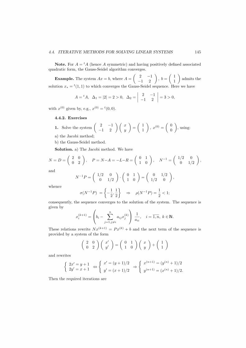
4.4. ITERATIVE METHODS FOR SOLVING LINEAR SYSTEMS 145
Note. For A = tA (hence A symmetric) and having positively defined associatedquadratic form, the Gauss-Seidel algorithm converges.
Example. The system Ax = b, where A =(
2 −1−1 2
), b =
(11
)admits the
solution x∗ = t(1, 1) to which converges the Gauss-Seidel sequence. Here we have
A = tA, ∆1 = |2| = 2 > 0, ∆2 =∣∣∣∣
2 −1−1 2
∣∣∣∣ = 3 > 0,
with x(0) given by, e.g., x(0) = t(0, 0).
4.4.2. Exercises
1. Solve the system(
2 −1−1 2
)(xy
)=
(11
), x(0) =
(00
), using:
a) the Jacobi method;b) the Gauss-Seidel method.
Solution. a) The Jacobi method. We have
N = D =(
2 00 2
), P = N−A = −L−R =
(0 11 0
), N−1 =
(1/2 00 1/2
),
and
N−1P =(
1/2 00 1/2
)·(
0 11 0
)=
(0 1/2
1/2 0
),
whence
σ(N−1P ) =−1
2,12
⇒ ρ(N−1P ) =
12
< 1;
consequently, the sequence converges to the solution of the system. The sequence isgiven by
x(k+1)i =
bi −
n∑
j=1,j 6=i
aijx(k)j
1
aii, i = 1, n, k ∈ N.
These relations rewrite Nx(k+1) = Px(k) + b and the next term of the sequence isprovided by a system of the form
(2 00 2
)(x′
y′
)=
(0 11 0
)(xy
)+
(11
)
and rewrites
2x′ = y + 12y′ = x + 1 ⇔
x′ = (y + 1)/2
y′ = (x + 1)/2⇒
x(n+1) = (y(n) + 1)/2
y(n+1) = (x(n) + 1)/2.
Then the required iterations are
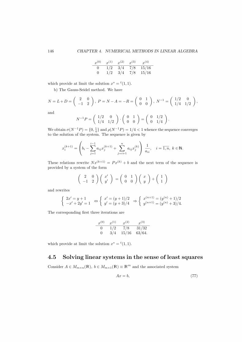
146 CHAPTER 4. NUMERICAL METHODS IN LINEAR ALGEBRA
x(0) x(1) x(2) x(3) x(4)
0 1/2 3/4 7/8 15/160 1/2 3/4 7/8 15/16
which provide at limit the solution x∗ = t(1, 1).
b) The Gauss-Seidel method. We have
N = L+D =(
2 0−1 2
), P = N −A = −R =
(0 10 0
), N−1 =
(1/2 01/4 1/2
),
and
N−1P =(
1/2 01/4 1/2
)·(
0 10 0
)=
(0 1/20 1/4
).
We obtain σ(N−1P ) = 0, 14 and ρ(N−1P ) = 1/4 < 1 whence the sequence converges
to the solution of the system. The sequence is given by
x(k+1)i =
bi −
i−1∑
j=1
aijx(k+1)j +
n∑
j=i+1
aijx(k)j
1
aii, i = 1, n, k ∈ N.
These relations rewrite Nx(k+1) = Px(k) + b and the next term of the sequence isprovided by a system of the form
(2 0−1 2
)(x′
y′
)=
(0 10 0
)(xy
)+
(11
)
and rewrites
2x′ = y + 1−x′ + 2y′ = 1 ⇔
x′ = (y + 1)/2y′ = (y + 3)/4 ⇒
x(n+1) = (y(n) + 1)/2y(n+1) = (y(n) + 3)/4.
The corresponding first three iterations are
x(0) x(1) x(2) x(3)
0 1/2 7/8 31/320 3/4 15/16 63/64.
which provide at limit the solution x∗ = t(1, 1).
4.5 Solving linear systems in the sense of least squares
Consider A ∈ Mm×n( R), b ∈ Mm×1( R) ≡ Rm and the associated system
Ax = b, (77)
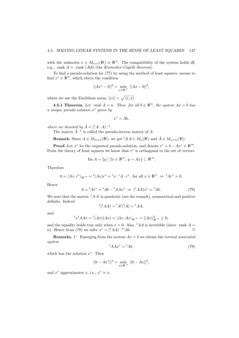
4.5. SOLVING LINEAR SYSTEMS IN THE SENSE OF LEAST SQUARES 147
with the unknown x ∈ Mn×1(R) ≡ Rn. The compatibility of the system holds iff,e.g., rank A = rank (A|b) (the Kronecker-Capelli theorem).
To find a pseudo-solution for (77) by using the method of least squares, means tofind x∗ ∈ Rn, which obeys the condition
||Ax∗ − b||2 = minx∈R
n||Ax− b||2,
where we use the Euclidean norm, ||x|| =√〈x, x〉.
4.5.1 Theorem. Let rank A = n. Then for all b ∈ Rn, the system Ax = b hasa unique pseudo-solution x∗ given by
x∗ = Ab,
where we denoted by A = (tA ·A)−1.The matrix A−1 is called the pseudo-inverse matrix of A.
Remark. Since A ∈ Mm×n( R), we get tA A ∈ Mn(R) and A ∈ Mn×m( R).
Proof. Let x∗ be the requested pseudo-solution, and denote r∗ = b−Ax∗ ∈ Rm.From the theory of least squares we know that r∗ is orthogonal to the set of vectors
Im A = y | ∃x ∈ Rn, y = Ax ⊂ Rm.
Therefore
0 = 〈Ax, r∗〉Rm = t(Ax)r∗ = tx · tA · r∗, for all x ∈ Rn ⇒ tAr∗ = 0.
Hence0 = tAr∗ = tAb− tAAx∗ ⇒ (tAA)x∗ = tAb. (78)
We note that the matrix tAA is quadratic (see the remark), symmetrical and positivedefinite. Indeed
t(tAA) = tAt(tA) = tAA,
andtxtAAx = t(Ax)(Ax) = 〈Ax,Ax〉R
m = ||Ax||2R m ≥ 0,
and the equality holds true only when x = 0. Also, tAA is invertible (since rank A =n). Hence from (78) we infer x∗ = (tAA)−1tAb. 2
Remarks. 1o. Emerging from the system Ax = b we obtain the normal associatedsystem
tAAx∗ = tAb, (79)
which has the solution x∗. Then
||b−Ax∗||2 = minx∈R
n||b−Ax||2,
and x∗ approximates x, i.e., x∗ ' x.
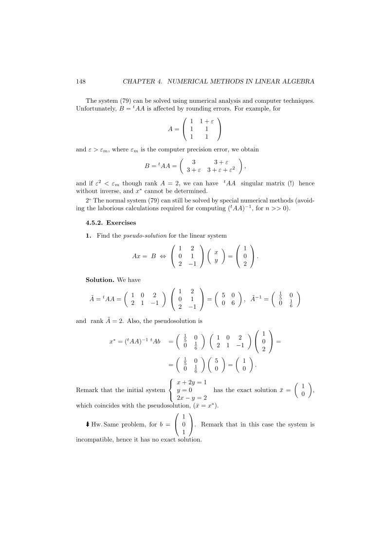
148 CHAPTER 4. NUMERICAL METHODS IN LINEAR ALGEBRA
The system (79) can be solved using numerical analysis and computer techniques.Unfortunately, B = tAA is affected by rounding errors. For example, for
A =
1 1 + ε1 11 1
and ε > εm, where εm is the computer precision error, we obtain
B = tAA =(
3 3 + ε3 + ε 3 + ε + ε2
),
and if ε2 < εm though rank A = 2, we can have tAA singular matrix (!) hencewithout inverse, and x∗ cannot be determined.
2o The normal system (79) can still be solved by special numerical methods (avoid-ing the laborious calculations required for computing (tAA)−1, for n >> 0).
4.5.2. Exercises
1. Find the pseudo-solution for the linear system
Ax = B ⇔
1 20 12 −1
(xy
)=
102
.
Solution. We have
A = tAA =(
1 0 22 1 −1
)
1 20 12 −1
=
(5 00 6
), A−1 =
(15 00 1
6
)
and rank A = 2. Also, the pseudosolution is
x∗ = (tAA)−1 tAb =(
15 00 1
6
) (1 0 22 1 −1
)
102
=
=(
15 00 1
6
)(50
)=
(10
).
Remark that the initial system
x + 2y = 1y = 02x− y = 2
has the exact solution x =(
10
),
which coincides with the pseudosolution, (x = x∗).
Hw. Same problem, for b =
101
. Remark that in this case the system is
incompatible, hence it has no exact solution.
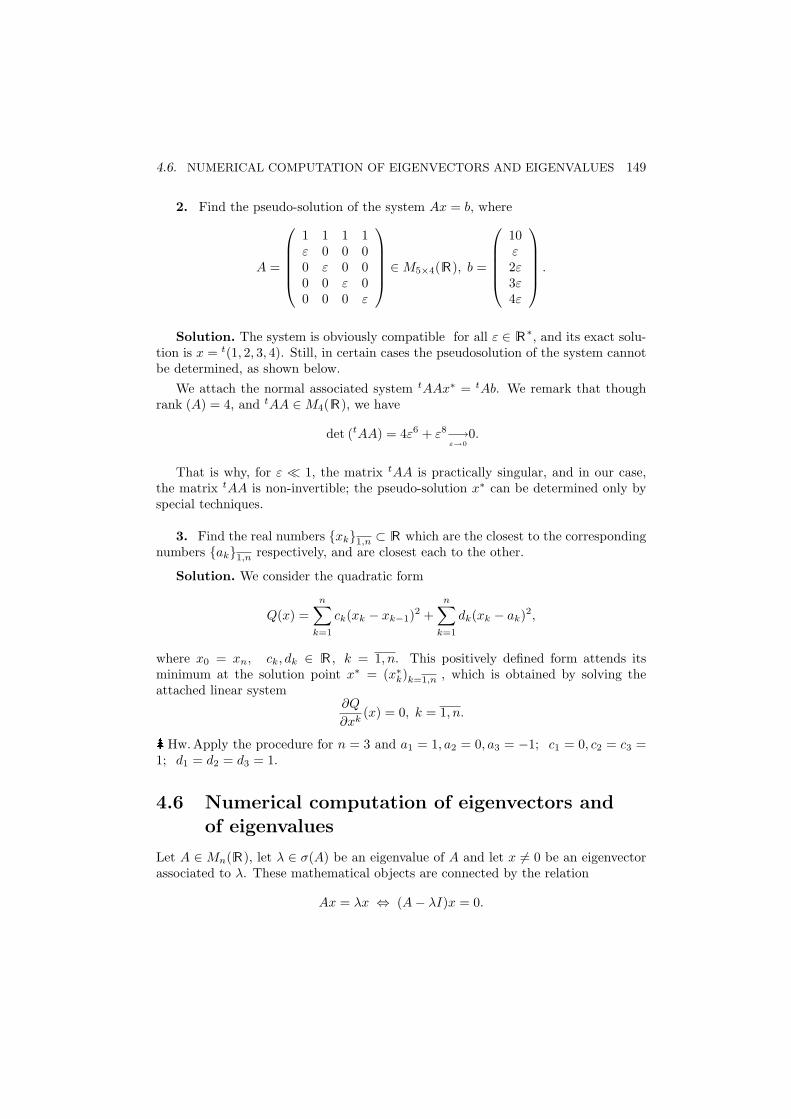
4.6. NUMERICAL COMPUTATION OF EIGENVECTORS AND EIGENVALUES 149
2. Find the pseudo-solution of the system Ax = b, where
A =
1 1 1 1ε 0 0 00 ε 0 00 0 ε 00 0 0 ε
∈ M5×4(R), b =
10ε2ε3ε4ε
.
Solution. The system is obviously compatible for all ε ∈ R∗, and its exact solu-tion is x = t(1, 2, 3, 4). Still, in certain cases the pseudosolution of the system cannotbe determined, as shown below.
We attach the normal associated system tAAx∗ = tAb. We remark that thoughrank (A) = 4, and tAA ∈ M4(R), we have
det (tAA) = 4ε6 + ε8−→ε→0
0.
That is why, for ε ¿ 1, the matrix tAA is practically singular, and in our case,the matrix tAA is non-invertible; the pseudo-solution x∗ can be determined only byspecial techniques.
3. Find the real numbers xk1,n ⊂ R which are the closest to the correspondingnumbers ak1,n respectively, and are closest each to the other.
Solution. We consider the quadratic form
Q(x) =n∑
k=1
ck(xk − xk−1)2 +n∑
k=1
dk(xk − ak)2,
where x0 = xn, ck, dk ∈ R , k = 1, n. This positively defined form attends itsminimum at the solution point x∗ = (x∗k)k=1,n , which is obtained by solving theattached linear system
∂Q
∂xk(x) = 0, k = 1, n.
Hw. Apply the procedure for n = 3 and a1 = 1, a2 = 0, a3 = −1; c1 = 0, c2 = c3 =1; d1 = d2 = d3 = 1.
4.6 Numerical computation of eigenvectors andof eigenvalues
Let A ∈ Mn(R), let λ ∈ σ(A) be an eigenvalue of A and let x 6= 0 be an eigenvectorassociated to λ. These mathematical objects are connected by the relation
Ax = λx ⇔ (A− λI)x = 0.
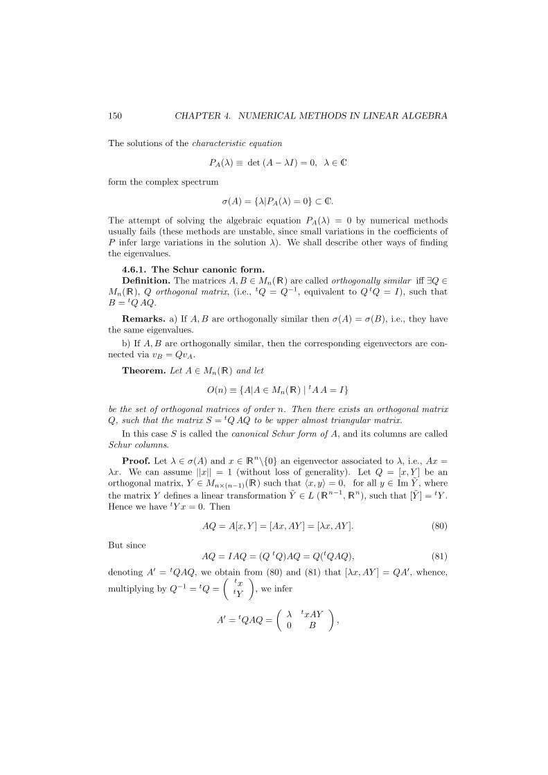
150 CHAPTER 4. NUMERICAL METHODS IN LINEAR ALGEBRA
The solutions of the characteristic equation
PA(λ) ≡ det (A− λI) = 0, λ ∈ C
form the complex spectrum
σ(A) = λ|PA(λ) = 0 ⊂ C.
The attempt of solving the algebraic equation PA(λ) = 0 by numerical methodsusually fails (these methods are unstable, since small variations in the coefficients ofP infer large variations in the solution λ). We shall describe other ways of findingthe eigenvalues.
4.6.1. The Schur canonic form.Definition. The matrices A, B ∈ Mn( R) are called orthogonally similar iff ∃Q ∈
Mn(R), Q orthogonal matrix, (i.e., tQ = Q−1, equivalent to Q tQ = I), such thatB = tQAQ.
Remarks. a) If A,B are orthogonally similar then σ(A) = σ(B), i.e., they havethe same eigenvalues.
b) If A,B are orthogonally similar, then the corresponding eigenvectors are con-nected via vB = QvA.
Theorem. Let A ∈ Mn(R) and let
O(n) ≡ A|A ∈ Mn( R) | tAA = Ibe the set of orthogonal matrices of order n. Then there exists an orthogonal matrixQ, such that the matrix S = tQAQ to be upper almost triangular matrix.
In this case S is called the canonical Schur form of A, and its columns are calledSchur columns.
Proof. Let λ ∈ σ(A) and x ∈ Rn\0 an eigenvector associated to λ, i.e., Ax =λx. We can assume ||x|| = 1 (without loss of generality). Let Q = [x, Y ] be anorthogonal matrix, Y ∈ Mn×(n−1)(R) such that 〈x, y〉 = 0, for all y ∈ Im Y , wherethe matrix Y defines a linear transformation Y ∈ L (Rn−1, Rn), such that [Y ] = tY .Hence we have tY x = 0. Then
AQ = A[x, Y ] = [Ax,AY ] = [λx,AY ]. (80)
But sinceAQ = IAQ = (Q tQ)AQ = Q(tQAQ), (81)
denoting A′ = tQAQ, we obtain from (80) and (81) that [λx,AY ] = QA′, whence,
multiplying by Q−1 = tQ =(
txtY
), we infer
A′ = tQAQ =(
λ txAY0 B
),
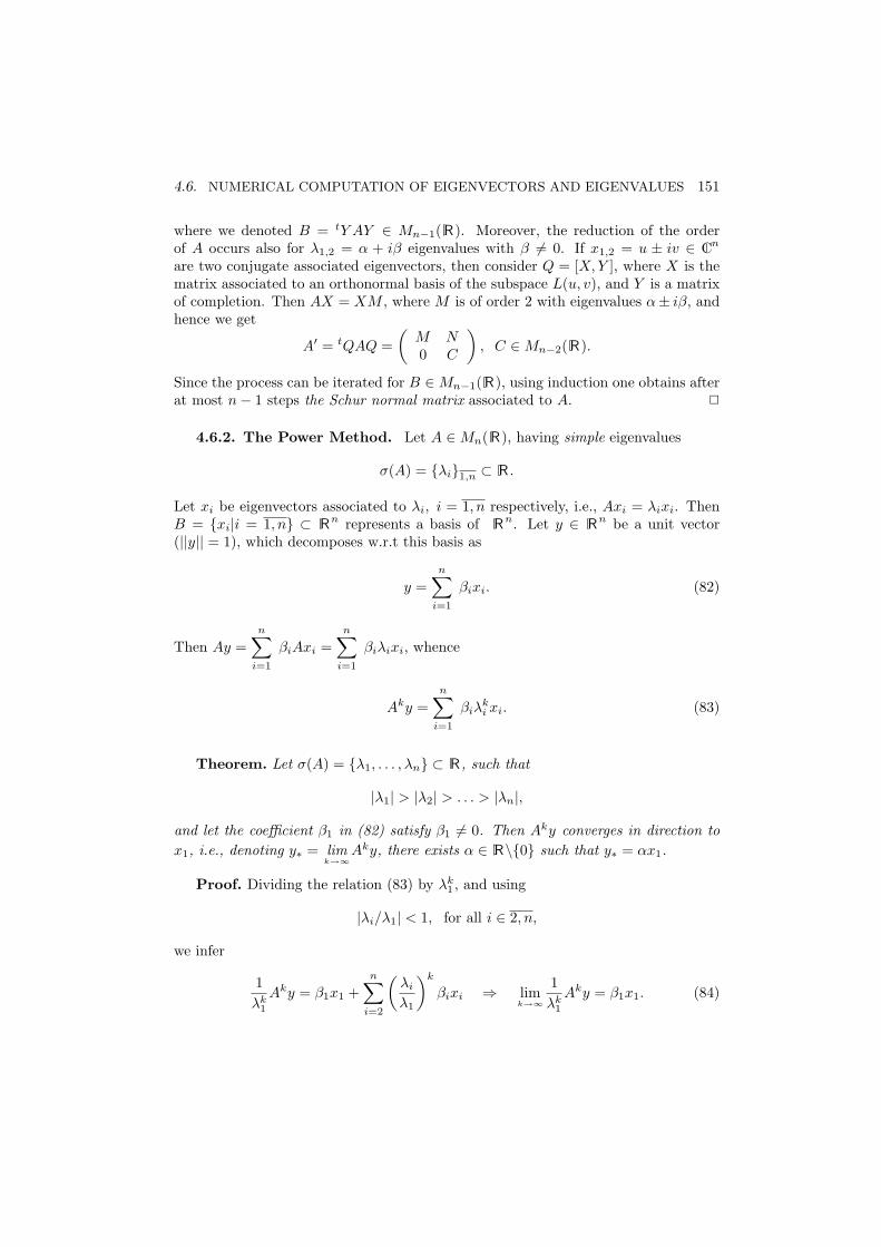
4.6. NUMERICAL COMPUTATION OF EIGENVECTORS AND EIGENVALUES 151
where we denoted B = tY AY ∈ Mn−1( R). Moreover, the reduction of the orderof A occurs also for λ1,2 = α + iβ eigenvalues with β 6= 0. If x1,2 = u ± iv ∈ Cn
are two conjugate associated eigenvectors, then consider Q = [X, Y ], where X is thematrix associated to an orthonormal basis of the subspace L(u, v), and Y is a matrixof completion. Then AX = XM , where M is of order 2 with eigenvalues α± iβ, andhence we get
A′ = tQAQ =(
M N0 C
), C ∈ Mn−2(R).
Since the process can be iterated for B ∈ Mn−1(R), using induction one obtains afterat most n− 1 steps the Schur normal matrix associated to A. 2
4.6.2. The Power Method. Let A ∈ Mn(R), having simple eigenvalues
σ(A) = λi1,n ⊂ R .
Let xi be eigenvectors associated to λi, i = 1, n respectively, i.e., Axi = λixi. ThenB = xi|i = 1, n ⊂ Rn represents a basis of Rn. Let y ∈ Rn be a unit vector(||y|| = 1), which decomposes w.r.t this basis as
y =n∑
i=1
βixi. (82)
Then Ay =n∑
i=1
βiAxi =n∑
i=1
βiλixi, whence
Aky =n∑
i=1
βiλki xi. (83)
Theorem. Let σ(A) = λ1, . . . , λn ⊂ R , such that
|λ1| > |λ2| > . . . > |λn|,
and let the coefficient β1 in (82) satisfy β1 6= 0. Then Aky converges in direction tox1, i.e., denoting y∗ = lim
k→∞Aky, there exists α ∈ R\0 such that y∗ = αx1.
Proof. Dividing the relation (83) by λk1 , and using
|λi/λ1| < 1, for all i ∈ 2, n,
we infer
1λk
1
Aky = β1x1 +n∑
i=2
(λi
λ1
)k
βixi ⇒ limk→∞
1λk
1
Aky = β1x1. (84)
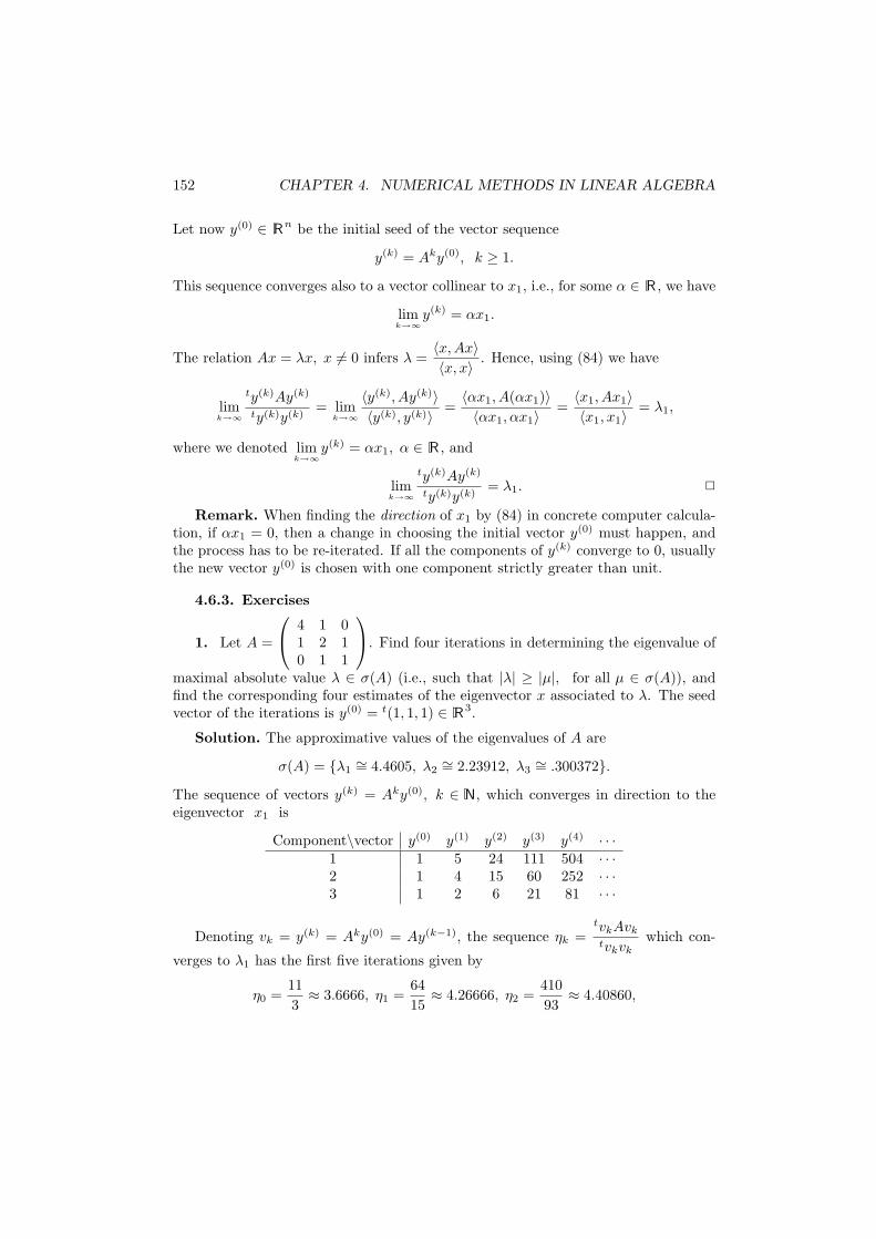
152 CHAPTER 4. NUMERICAL METHODS IN LINEAR ALGEBRA
Let now y(0) ∈ Rn be the initial seed of the vector sequence
y(k) = Aky(0), k ≥ 1.
This sequence converges also to a vector collinear to x1, i.e., for some α ∈ R , we have
limk→∞
y(k) = αx1.
The relation Ax = λx, x 6= 0 infers λ =〈x,Ax〉〈x, x〉 . Hence, using (84) we have
limk→∞
ty(k)Ay(k)
ty(k)y(k)= lim
k→∞
〈y(k), Ay(k)〉〈y(k), y(k)〉 =
〈αx1, A(αx1)〉〈αx1, αx1〉 =
〈x1, Ax1〉〈x1, x1〉 = λ1,
where we denoted limk→∞
y(k) = αx1, α ∈ R , and
limk→∞
ty(k)Ay(k)
ty(k)y(k)= λ1. 2
Remark. When finding the direction of x1 by (84) in concrete computer calcula-tion, if αx1 = 0, then a change in choosing the initial vector y(0) must happen, andthe process has to be re-iterated. If all the components of y(k) converge to 0, usuallythe new vector y(0) is chosen with one component strictly greater than unit.
4.6.3. Exercises
1. Let A =
4 1 01 2 10 1 1
. Find four iterations in determining the eigenvalue of
maximal absolute value λ ∈ σ(A) (i.e., such that |λ| ≥ |µ|, for all µ ∈ σ(A)), andfind the corresponding four estimates of the eigenvector x associated to λ. The seedvector of the iterations is y(0) = t(1, 1, 1) ∈ R3.
Solution. The approximative values of the eigenvalues of A are
σ(A) = λ1∼= 4.4605, λ2
∼= 2.23912, λ3∼= .300372.
The sequence of vectors y(k) = Aky(0), k ∈ N, which converges in direction to theeigenvector x1 is
Component\vector y(0) y(1) y(2) y(3) y(4) · · ·1 1 5 24 111 504 · · ·2 1 4 15 60 252 · · ·3 1 2 6 21 81 · · ·
Denoting vk = y(k) = Aky(0) = Ay(k−1), the sequence ηk =tvkAvk
tvkvkwhich con-
verges to λ1 has the first five iterations given by
η0 =113≈ 3.6666, η1 =
6415≈ 4.26666, η2 =
41093
≈ 4.40860,
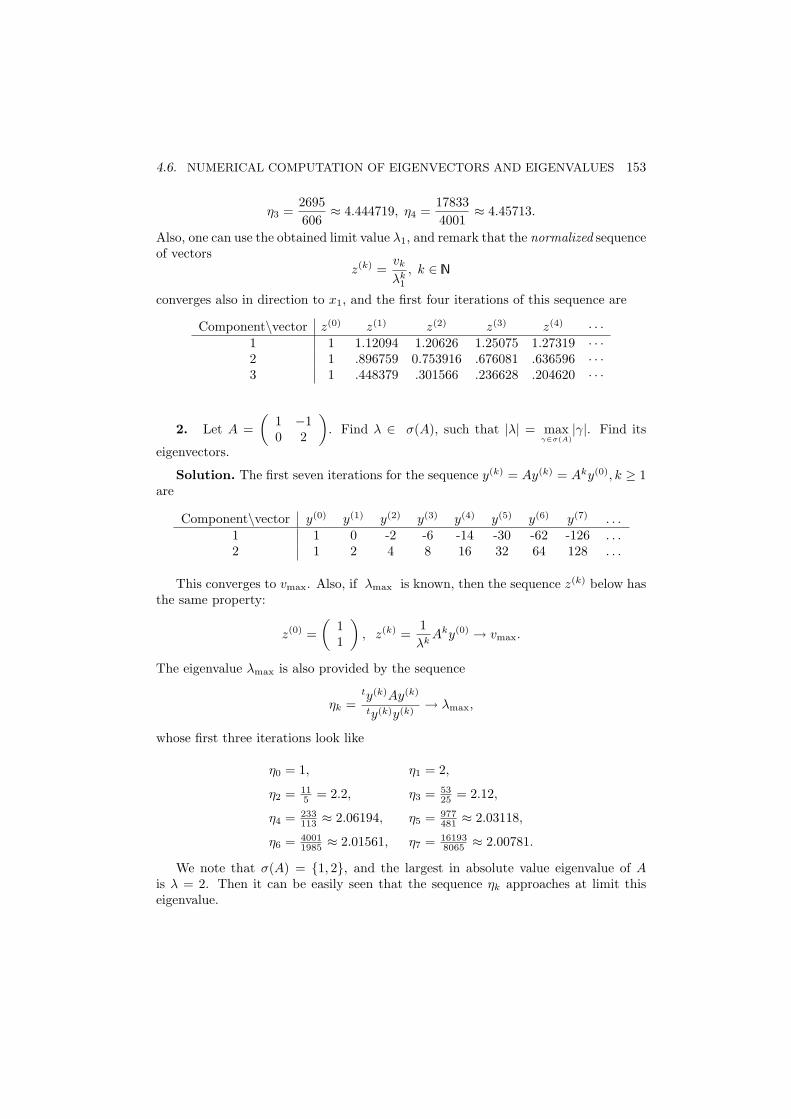
4.6. NUMERICAL COMPUTATION OF EIGENVECTORS AND EIGENVALUES 153
η3 =2695606
≈ 4.444719, η4 =178334001
≈ 4.45713.
Also, one can use the obtained limit value λ1, and remark that the normalized sequenceof vectors
z(k) =vk
λk1
, k ∈ N
converges also in direction to x1, and the first four iterations of this sequence are
Component\vector z(0) z(1) z(2) z(3) z(4) · · ·1 1 1.12094 1.20626 1.25075 1.27319 · · ·2 1 .896759 0.753916 .676081 .636596 · · ·3 1 .448379 .301566 .236628 .204620 · · ·
2. Let A =(
1 −10 2
). Find λ ∈ σ(A), such that |λ| = max
γ∈σ(A)|γ|. Find its
eigenvectors.
Solution. The first seven iterations for the sequence y(k) = Ay(k) = Aky(0), k ≥ 1are
Component\vector y(0) y(1) y(2) y(3) y(4) y(5) y(6) y(7) . . .1 1 0 -2 -6 -14 -30 -62 -126 . . .2 1 2 4 8 16 32 64 128 . . .
This converges to vmax. Also, if λmax is known, then the sequence z(k) below hasthe same property:
z(0) =(
11
), z(k) =
1λk
Aky(0) → vmax.
The eigenvalue λmax is also provided by the sequence
ηk =ty(k)Ay(k)
ty(k)y(k)→ λmax,
whose first three iterations look like
η0 = 1, η1 = 2,
η2 = 115 = 2.2, η3 = 53
25 = 2.12,
η4 = 233113 ≈ 2.06194, η5 = 977
481 ≈ 2.03118,
η6 = 40011985 ≈ 2.01561, η7 = 16193
8065 ≈ 2.00781.
We note that σ(A) = 1, 2, and the largest in absolute value eigenvalue of Ais λ = 2. Then it can be easily seen that the sequence ηk approaches at limit thiseigenvalue.
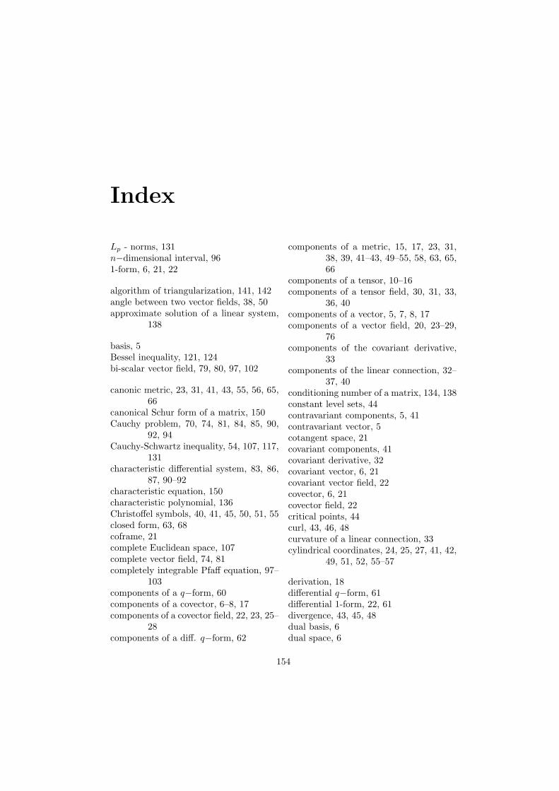
Index
Lp - norms, 131n−dimensional interval, 961-form, 6, 21, 22
algorithm of triangularization, 141, 142angle between two vector fields, 38, 50approximate solution of a linear system,
138
basis, 5Bessel inequality, 121, 124bi-scalar vector field, 79, 80, 97, 102
canonic metric, 23, 31, 41, 43, 55, 56, 65,66
canonical Schur form of a matrix, 150Cauchy problem, 70, 74, 81, 84, 85, 90,
92, 94Cauchy-Schwartz inequality, 54, 107, 117,
131characteristic differential system, 83, 86,
87, 90–92characteristic equation, 150characteristic polynomial, 136Christoffel symbols, 40, 41, 45, 50, 51, 55closed form, 63, 68coframe, 21complete Euclidean space, 107complete vector field, 74, 81completely integrable Pfaff equation, 97–
103components of a q−form, 60components of a covector, 6–8, 17components of a covector field, 22, 23, 25–
28components of a diff. q−form, 62
components of a metric, 15, 17, 23, 31,38, 39, 41–43, 49–55, 58, 63, 65,66
components of a tensor, 10–16components of a tensor field, 30, 31, 33,
36, 40components of a vector, 5, 7, 8, 17components of a vector field, 20, 23–29,
76components of the covariant derivative,
33components of the linear connection, 32–
37, 40conditioning number of a matrix, 134, 138constant level sets, 44contravariant components, 5, 41contravariant vector, 5cotangent space, 21covariant components, 41covariant derivative, 32covariant vector, 6, 21covariant vector field, 22covector, 6, 21covector field, 22critical points, 44curl, 43, 46, 48curvature of a linear connection, 33cylindrical coordinates, 24, 25, 27, 41, 42,
49, 51, 52, 55–57
derivation, 18differential q−form, 61differential 1-form, 22, 61divergence, 43, 45, 48dual basis, 6dual space, 6
154
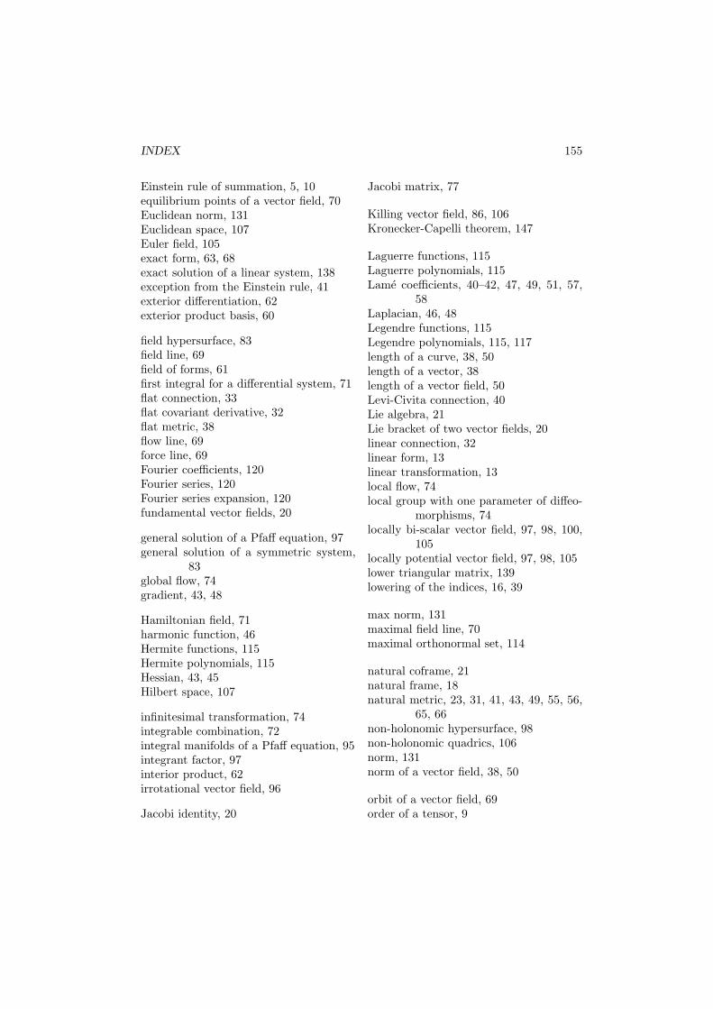
INDEX 155
Einstein rule of summation, 5, 10equilibrium points of a vector field, 70Euclidean norm, 131Euclidean space, 107Euler field, 105exact form, 63, 68exact solution of a linear system, 138exception from the Einstein rule, 41exterior differentiation, 62exterior product basis, 60
field hypersurface, 83field line, 69field of forms, 61first integral for a differential system, 71flat connection, 33flat covariant derivative, 32flat metric, 38flow line, 69force line, 69Fourier coefficients, 120Fourier series, 120Fourier series expansion, 120fundamental vector fields, 20
general solution of a Pfaff equation, 97general solution of a symmetric system,
83global flow, 74gradient, 43, 48
Hamiltonian field, 71harmonic function, 46Hermite functions, 115Hermite polynomials, 115Hessian, 43, 45Hilbert space, 107
infinitesimal transformation, 74integrable combination, 72integral manifolds of a Pfaff equation, 95integrant factor, 97interior product, 62irrotational vector field, 96
Jacobi identity, 20
Jacobi matrix, 77
Killing vector field, 86, 106Kronecker-Capelli theorem, 147
Laguerre functions, 115Laguerre polynomials, 115Lame coefficients, 40–42, 47, 49, 51, 57,
58Laplacian, 46, 48Legendre functions, 115Legendre polynomials, 115, 117length of a curve, 38, 50length of a vector, 38length of a vector field, 50Levi-Civita connection, 40Lie algebra, 21Lie bracket of two vector fields, 20linear connection, 32linear form, 13linear transformation, 13local flow, 74local group with one parameter of diffeo-
morphisms, 74locally bi-scalar vector field, 97, 98, 100,
105locally potential vector field, 97, 98, 105lower triangular matrix, 139lowering of the indices, 16, 39
max norm, 131maximal field line, 70maximal orthonormal set, 114
natural coframe, 21natural frame, 18natural metric, 23, 31, 41, 43, 49, 55, 56,
65, 66non-holonomic hypersurface, 98non-holonomic quadrics, 106norm, 131norm of a vector field, 38, 50
orbit of a vector field, 69order of a tensor, 9
156 INDEX
order of contravariance, 9order of covariance, 9orthogonal coordinates, 40orthogonal matrix, 150orthogonal projection, 109orthogonal set, 114orthogonal vector fields, 38orthogonally similar matrices, 150orthonormal basis, 38, 114orthonormal set, 114
parallel tensor field, 34parallel vector field, 93Parseval equality, 120physical comp. of the gradient, 48physical components, 41Poincare metric, 38, 50, 58Poincare plane, 50, 58polar coordinates, 28, 29, 31, 51potential vector field, 97principal submatrices of a matrix, 139product basis, 30pseudo-inverse matrix of a matrix, 147pseudo-solution, 148Pythagorean theorem, 109
raising of the indices, 16, 39reciprocal tensor field of a metric, 39, 50relative error, 138representation of a linear functional, 126Riemannian manifold, 38Riemannian metric, 15, 38rotor, 43, 46, 48rounding error, 138
scalar, 13scalar field, 17scalar product of two vector fields, 38scalar product on Cn, 108scalar product on L2, 108scalar product on l2, 108scalar product on Rn, 108scalar product on V3, 108scalar product on C0[a, b], 108Schur canonic form, 150
Schur columns, 150Schur normal matrix, 151singular points, 98sky-scrapper norm, 131spectral radius of a matrix, 136speed, 50spherical coordinates, 24, 27, 28, 41, 49,
51, 52, 55, 56, 58steepest increase of a function, 44, 53, 54symmetric system, 72symmetrical connection, 33, 36
tangent vector, 18tensor field, 29tensor of type (p, q), 9tensor product, 9torsion of a linear connection, 33transvection of tensors, 11triangle inequality, 131
unconditionally convergent series, 123upper triangular matrix, 139
variation of a function along a given di-rection, 54
vector field, 17, 19–21, 23, 24, 26–28, 32,38, 40, 43, 48–52, 54, 55, 57, 63,69–71, 74–77, 79–82, 86, 88, 91–98, 100–102, 105
velocity, 50volume element, 48
zeros of a vector field, 70

Bibliography
[1] I.S.Antoniu, Calculul matricial si tensorial ın electrotehnica (in Romanian), Ed.Tehnica, Bucharest, 1962.
[2] T.M.Apostol, Calculus, vol. II, Blaisdell Publishing Company, 1969.
[3] V.Balan, Algebra liniara, geometrie analitica (in Romanian), Fair Partners Eds.,1999.
[4] V.Balan, I-R.Nicola, Algebra liniara, geometrie analitica si diferentiala, ecuatiidiferentiale (in Romanian), Bren Eds., Bucharest2004, 2006.
[5] I.Beju, O.Soos, P.P.Teodorescu, Tehnici de calcul spinorial si tensorial neeuclid-ian cu aplicatii (in Romanian), Ed. Tehnica, Bucharest, 1968.
[6] M.Berger, B.Gostiaux, Geometrie differentielle, Armand Colin, Paris, 1972.
[7] G.Berman, Problemes d’analyse mathematique, Editions de Moscou, 1976.
[8] R.M.Bowen, C.C.Wang, Introduction to Vectors and Tensors, vol. 1-2, PlenumPress, New York, 1976.
[9] F.Brickell, R.S.Clark, Differentiable Manifolds, Van Nostrand Reinhold Com-pany, London, 1970.
[10] B.M.Budak, S.V.Fomin, Multiple Integrals. Field Theory and Series, Mir Pub-lishers, Moskow, 1973.
[11] S.Chirita, Probleme de matematici superioare (in Romanian), Ed. Did. Ped.,Bucharest, 1989.
[12] C.Dragusin, L.Dragusin, Analiza matematica, vol. II, (in Romanian), Ed. MatrixRom, Bucharest, 1999.
[13] B.Dubrovin, S.Novikov, A.Fomenko, Geometria Contemporanea, Editori Riuniti,Edizioni Mir, 1987.
[14] G.M.Fihtenholt, Curs de calcul diferential si integral, vol. 3 (in Romanian), Ed.Tehnica, Bucharest, 1965.
157
158 BIBLIOGRAPHY
[15] Gh. Gheorghiev, V. Oproiu, Geometrie diferentiala (in Romanian), Ed. Did.Ped., Bucharest, 1977.
[16] I.Glazman, Iu.Liubici, Analiza liniara pe spatii finit dimensionale (in Romanian),Ed. St. Encicl., Bucharest, 1980; Nauka Eds (in Russian), 1969.
[17] J.N.Harris, H.Stocker, Handbook of Mathematics and Computational Sciences,Springer Verlag, 1998.
[18] S.Helgason, Differential Geometry and Symmetric Spaces, Academic Press, 1962.
[19] R.Hermann, Topics in Physical Geometry, Topics in Physical Geometry, v.26,Mathematical Science Press, Brooklin, 1988.
[20] S.Ianus, Geometrie diferentiala cu aplicatii ın teoria relativitatii (in Romanian),Academy Eds., Bucharest, 1983.
[21] W.Klingenberg, Lineare Algebra und Geometrie, Springer-Verlag, Berlin, 1990.
[22] N.E.Kocin, Calculul vectorial si introducere ın calculul tensorial (in Romanian),Ed. Tehnica, Bucharest, 1954.
[23] I.A.Kostrikin, I.Yu.Manin, Linear Algebra and Geometry, Gordon and BreachScience Publishers, 1989.
[24] N.I.Kovantzov, G.M.Zrajevskaya, V.G.Kotcharovski, V.I.Mihailovski, ProblemBook in Differential Geometry and Topology (in Russian), Visha Shkola Eds.,Kiev, 1989.
[25] S.Lang, Differential and Riemannian Manifolds, GTM 160, Springer Verlag,1998.
[26] A.Lichnerowicz, Algebre et analyse lineaire, Masson & Cie, Paris, 1960.
[27] R.Millman, G.Parker, Elements of Differential Geometry, Prentice- Hall, Inc.,New Jersey, 1977.
[28] A.S.Mischenko, Iu.P.Soloviev, A.T.Fomenko, Problem book on Differential Ge-ometry and Topology (in Russian), University of Moskow, 1981.
[29] Gh.Munteanu, V.Balan, Lectii de teoria relativitatii (in Romanian), Bren Eds.,Bucharest, 2000.
[30] A.W.Naylor, G.R.Sell, Linear operator theory in engineering and science,Springer-Verlag, 1982.
[31] L.Nicolescu, Lectii de geometrie (in Romanian), Univ. Bucuresti, Bucharest,1990.
[32] V.Olariu, V.Prepelita, Teoria distributiilor, functii complexe si aplicatii, Ed. St.Encicl., Bucharest, 1986.
BIBLIOGRAPHY 159
[33] B. O’Neill, Elementary Differential Geometry, Academic Press, Fourth Printing,1970.
[34] P.V.O′Neill, Advanced Engineering Mathematics, Wadsworth Eds., 1991.
[35] D. Papuc, Geometrie diferentiala (in Romanian), Ed. Did. Ped., Bucharest, 1982.
[36] D. Papuc, I. D. Albu, Elemente de geometrie diferentiala globala (in Romanian),cap. I, II. 1, II. 4, VII. 2, Ed. Did. Ped., Bucharest, 1973,
[37] G.Pavel, F.I.Tomita, I.Gavrea, Matematici speciale. Aplicatii (in Romanian), Ed.Dacia, Cluj-Napoca, 1981.
[38] I. Popescu, Probleme de matematici superioare (in Romanian), Ed. Did. Ped.,Bucharest, 1964.
[39] C.Radu, C.Dragusin, L.Dragusin, Algebra liniara, analiza matematica, geometrieanalitica si diferentiala (culegere de probleme) (in Romanian), Ed.Fair Partners,Bucharest, 2000.
[40] C.Radu, C.Dragusin, L.Dragusin, Aplicatii de algebra, geometrie si matematicispeciale (in Romanian), Ed. Did. Ped., Bucharest, 1991.
[41] L.D.Raigorodski, P.C.Stavrinos, V.Balan, Introduction to the Physical Principlesof Differential Geometry, University of Athens, 1999.
[42] W.Rudin, Analiza reala si complexa (in Romanian), Ed. Theta, Bucharest, 1999.
[43] V.Rudner, C.Nicolescu, Probleme de matematici speciale (in Romanian), Ed.Did. Ped., Bucharest, 1982.
[44] B.Spain, Tensor Calculus, Central Book Co., Dublin, 1953.
[45] St. Staicu, Aplicatii ale calculului matriceal ın mecanica solidelor (in Romanian),Academy Eds., Bucharest, 1986.
[46] St. Staicu, Mecanica teoretica (in Romanian), Ed. Did. Ped., Bucharest, 1998.
[47] L.Stoica, Elements of Differentiable Manifolds, Geometry Balkan Press, Bu-curesti, Romania, 1998.
[48] K.Teleman, Introducere ın geometria diferentiala (in Romanian), Univ. Bu-curesti, Bucharest, 1986.
[49] J.A.Thorpe, Elementary Topics in Differential Geometry, Springer-Verlag, 1979.
[50] C.Udriste, Linii de camp (in Romanian), Ed. Tehnica, Bucharest, 1988.
[51] C.Udriste, Geometric Dynamics, Kluwer Academic Publishers, 2000.
[52] C.Udriste, Problems of Algebra, Geometry and Differential Equations I, II, Uni-versity Politehnica of Bucharest, Bucharest, 1992.
160 BIBLIOGRAPHY
[53] C.Udriste, Aplicatii de algebra, geometrie si ecuatii diferentiale (in Romanian),Ed. Did. Ped., Bucharest, 1993.
[54] C.Udriste, Algebra liniara, geometrie analitica (in Romanian), Geometry BalkanPress, Bucharest, 2000.
[55] C.Udriste, Geometrie diferentiala, ecuatii diferentiale (in Romanian), GeometryBalkan Press, Bucharest, 1997.
[56] C.Udriste, Problems of Linear Algebra, Analytic and Differential Geometry andDifferential Equations, Geometry Balkan Press, Bucharest, 2000.
[57] C.Udriste, V.Iftode, M.Postolache, Metode numerice de calcul (in Romanian),Ed. Tehnica, Bucharest, 1996.
[58] C.Udriste, C.Radu, C.Dicu, O.Malancioiu, Probleme de algebra, geometrie siecuatii diferentiale (in Romanian), Ed. Did. Ped., Bucharest, 1981.
[59] C.Udriste, C.Radu, C.Dicu, O.Malancioiu, Algebra, geometrie si ecuatiidiferentiale (in Romanian), Ed. Did. Ped., Bucharest, 1982.
[60] E.C.Young, Vector and Tensor Analysis, Pure and Applied Mathematics 172,M.Dekker, 1992.


