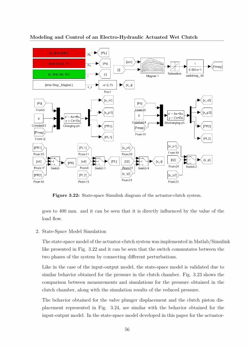
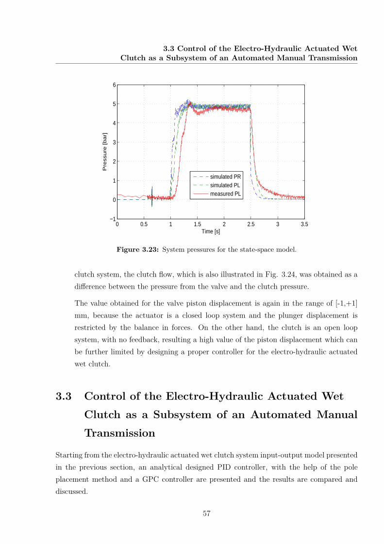
UNIVERSITATEA TEHNICĂ “GHEORGHE ASACHI” DIN IAŞI Şcoala Doctorală a Facultăţii de Automatică şi Calculatoare OVERALL POWERTRAIN MODELING AND CONTROL BASED ON DRIVELINE SUBSYSTEMS INTEGRATION (Controlul integrat al lanțului de transmisie a puterii) - TEZĂ DE DOCTORAT - Conducător de doctorat: Prof. univ. dr. ing. Corneliu Lazăr Doctorand: Ing. Andreea Elena Bălău IAŞI - 2011
Transcript
UNIVERSITATEA TEHNICĂ
“GHEORGHE ASACHI” DIN IAŞI
Şcoala Doctorală a Facultăţii de
Automatică şi Calculatoare
OVERALL POWERTRAIN MODELING AND CONTROL BASED ON DRIVELINE
SUBSYSTEMS INTEGRATION
(Controlul integrat al lanțului de transmisie a puterii)
- TEZĂ DE DOCTORAT -
Conducător de doctorat:
Prof. univ. dr. ing. Corneliu Lazăr
Doctorand:
Ing. Andreea Elena Bălău
IAŞI - 2011
UNIUNEA EUROPEANĂ GUVERNUL ROMÂNIEI
MINISTERUL MUNCII, FAMILIEI ŞI PROTECŢIEI SOCIALE
AMPOSDRU
Fondul Social European POSDRU 2007-2013
Instrumente Structurale 2007-2013
OIPOSDRU UNIVERSITATEA TEHNICĂ “GHEORGHE ASACHI”
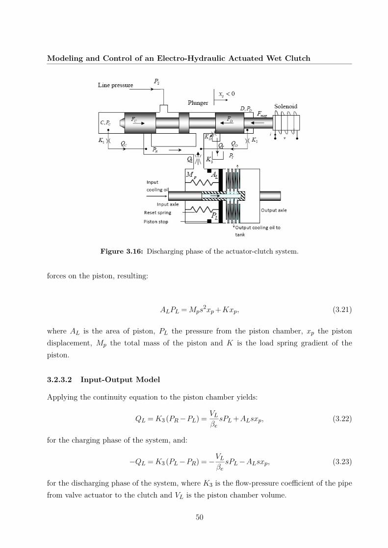
DIN IAŞI
UNIVERSITATEA TEHNICĂ “GHEORGHE ASACHI” DIN IAŞI
Şcoala Doctorală a Facultăţii de Automatică şi Calculatoare
OVERALL POWERTRAIN MODELING AND CONTROL BASED ON DRIVELINE
SUBSYSTEMS INTEGRATION (Controlul integrat al lanțului
de transmisie a puterii) - TEZĂ DE DOCTORAT -
Conducător de doctorat: Prof. univ. dr. ing. Corneliu Lazăr
Doctorand: Ing. Andreea Elena Bălău
IAŞI - 2011
UNIUNEA EUROPEANĂ GUVERNUL ROMÂNIEI
MINISTERUL MUNCII, FAMILIEI ŞI PROTECŢIEI SOCIALE
AMPOSDRU
Fondul Social European POSDRU 2007-2013
Instrumente Structurale 2007-2013
OIPOSDRU UNIVERSITATEA TEHNICĂ “GHEORGHE ASACHI”
DIN IAŞI
Teza de doctorat a fost realizată cu sprijinul financiar al
proiectului „Burse Doctorale - O Investiţie în Inteligenţă (BRAIN)”.
Proiectul „Burse Doctorale - O Investiţie în Inteligenţă (BRAIN)”,
POSDRU/6/1.5/S/9, ID 6681, este un proiect strategic care are ca
obiectiv general „Îmbunătățirea formării viitorilor cercetători în cadrul
ciclului 3 al învățământului superior - studiile universitare de doctorat
- cu impact asupra creșterii atractivității şi motivației pentru cariera în
cercetare”.
Proiect finanţat în perioada 2008 - 2011.
Finanţare proiect: 14.424.856,15 RON
Beneficiar: Universitatea Tehnică “Gheorghe Asachi” din Iaşi
Partener: Universitatea “Vasile Alecsandri” din Bacău
Director proiect: Prof. univ. dr. ing. Carmen TEODOSIU
Responsabil proiect partener: Prof. univ. dr. ing. Gabriel LAZĂR
UNIUNEA EUROPEANĂ GUVERNUL ROMÂNIEI
MINISTERUL MUNCII, FAMILIEI ŞI PROTECŢIEI SOCIALE
AMPOSDRU
Fondul Social European POSDRU 2007-2013
Instrumente Structurale 2007-2013
OIPOSDRU UNIVERSITATEA TEHNICĂ “GHEORGHE ASACHI”
DIN IAŞI
Motto:
Learn from yesterday, live for today, hope for tomorrow. The important thing is not to stop questioning.
Albert Einstein
UNIUNEA EUROPEANĂ GUVERNUL ROMÂNIEI
MINISTERUL MUNCII, FAMILIEI ŞI PROTECŢIEI SOCIALE
AMPOSDRU
Fondul Social European POSDRU 2007-2013
Instrumente Structurale 2007-2013
OIPOSDRU UNIVERSITATEA TEHNICĂ “GHEORGHE ASACHI”
DIN IAŞI
Acknowledgements
Looking back, I am surprised and at the same time very grateful for everythingI have received throughout these years. It has certainly shaped me as a personand has led me where I am now.
Foremost, I would like to express my sincere gratitude to my advisor Prof. Cor-neliu Lazăr, for the continuous support of my Ph.D study and research, for hismotivation, enthusiasm, patience and immense knowledge. His guidance helpedme in all the time of research and writing of this thesis.
My sincere thanks also goes to Prof. Paul van den Bosch and Asst. Prof. MirceaLazăr, for offering me the opportunity to work in their department, for the de-tailed and constructive comments and for the kind support and guidance thathave been of great value in this study. Also, I would like to thank Dr. ing.Stefano Di Cairano for the constructive discussions and advices.
I wish to express my warm thanks to Prof. Octavian Păstrăvănu, Prof. MihaelaHanako-Matcovski, Prof. Alexandru Onea, Assoc. Prof. Letiţia Mirea andAssoc. Prof. Lavinia Ferariu, for the extensive discussions around my work,constructive questions and excellent advices. I have to thank Costi for the sti-mulating discussions and for all the times we have worked together on variouspapers, and I also appreciate the short but productive collaboration I have hadwith Cristina.
It was a pleasure to share doctoral studies and life with wonderful people likeAdrian, Simona, Marius and Alex, my first office mates, and with my Ph.Dcolleagues Alina, Costi, Cosmin, Carlos and Bogdan, who are now my very closefriends. I will never forget Dana’s late night dinners and all the special momentsI have spent with Nicu. I would like to thank all of them for their friendshipand for sharing the glory and sadness of reports and conferences deadlines andday-to-day research, and also for all the fun we have had in the last three years.
I am forever indebted to my parents Mariana and Gheorghe, who raised me witha love of science and supported me in all my pursuits. I want to thank all of my
family for their understanding, their endless patience and encouragement whenit was most required, with a special thanks to my grandmother Paraschiva andmy sister Oana, for everything they have done for me. Finally, I want to dedicatethis thesis to my nephew Rivano, who I most love. He has shown a strong intereston studying when, at the early age of three, he clearly pointed out his interest ofbecoming a Professor Doctor Engineer.
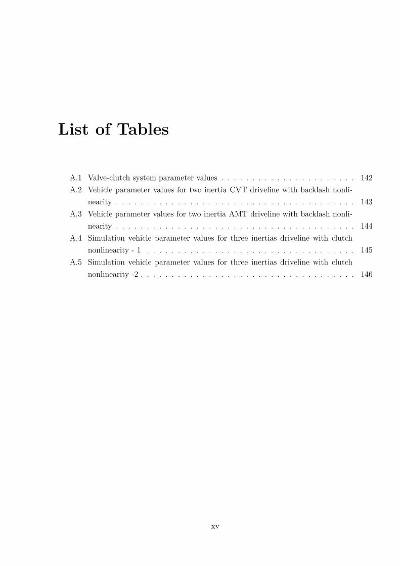
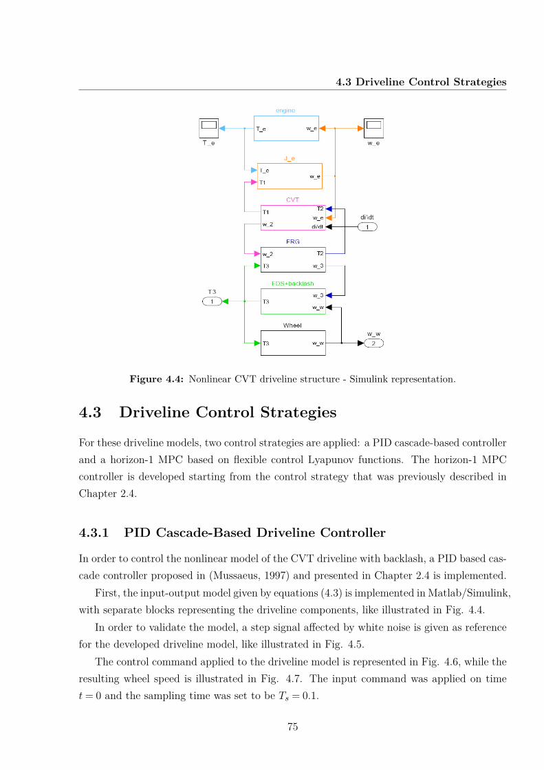
4.4.1 Simulator for the PWA Model of the CVT Driveline . . . . . . . . . . 804.4.2 Simulator for the Nonlinear Model of the CVT Driveline . . . . . . . 83
3.1 a) Test bench b) Schematic diagram . . . . . . . . . . . . . . . . . . . . . . . 333.2 a) Section through a real three stage pressure reducing valve; b) Three stage
valve schematic representation; c) Charging phase of the pressure reducingvalve; d) Discharging phase of the pressure reducing valve. . . . . . . . . . . 35
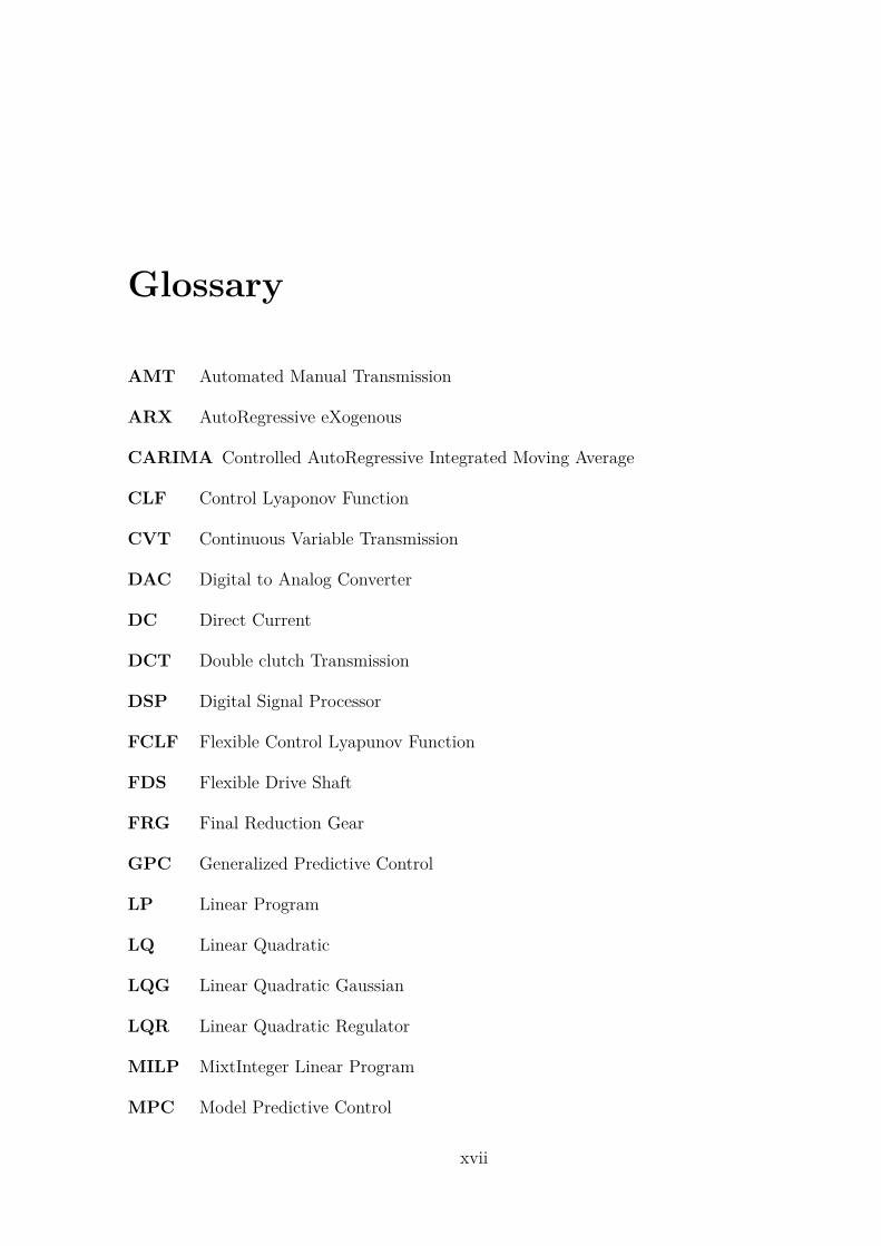
CARIMA Controlled AutoRegressive Integrated Moving Average
CLF Control Lyaponov Function
CVT Continuous Variable Transmission
DAC Digital to Analog Converter
DC Direct Current
DCT Double clutch Transmission
DSP Digital Signal Processor
FCLF Flexible Control Lyapunov Function
FDS Flexible Drive Shaft
FRG Final Reduction Gear
GPC Generalized Predictive Control
LP Linear Program
LQ Linear Quadratic
LQG Linear Quadratic Gaussian
LQR Linear Quadratic Regulator
MILP MixtInteger Linear Program
MPC Model Predictive Control
xvii
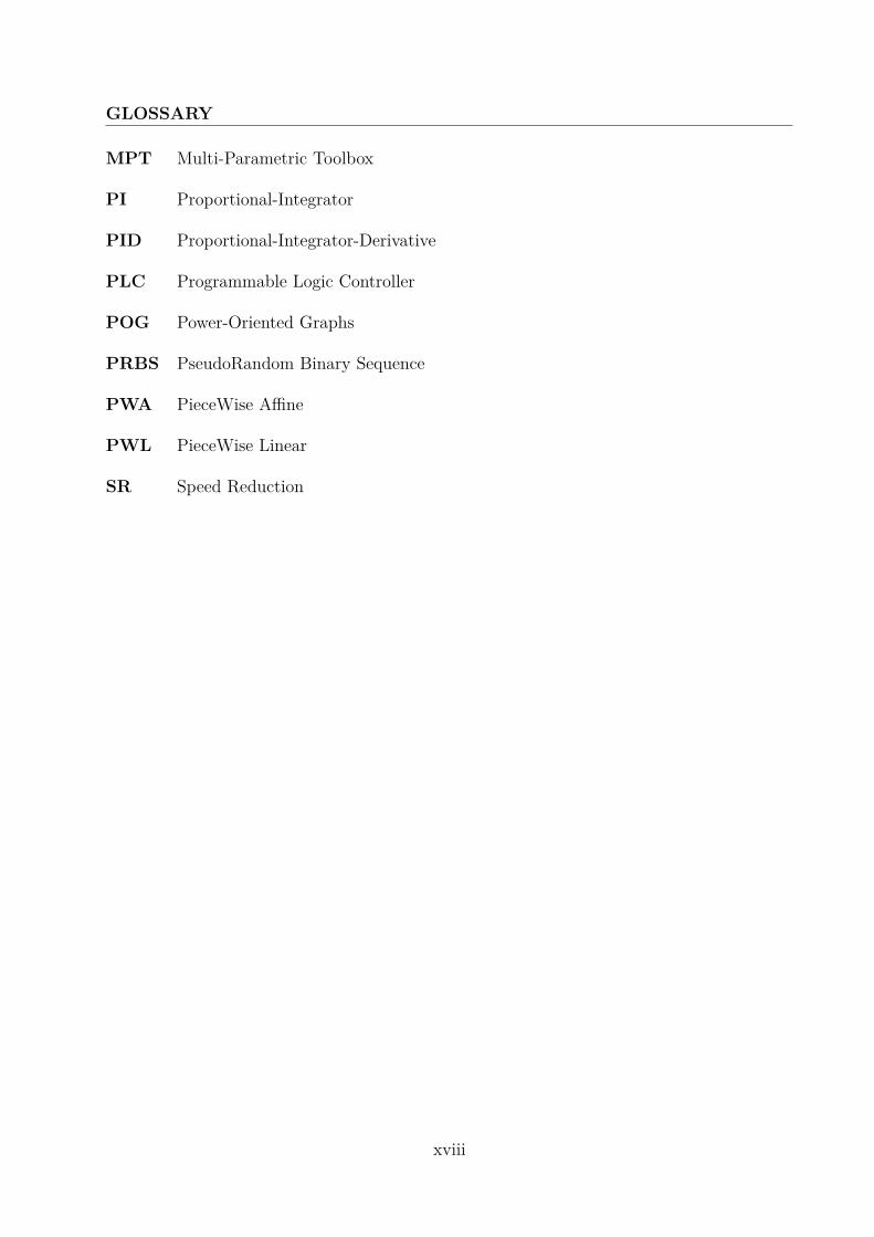
GLOSSARY
MPT Multi-Parametric Toolbox
PI Proportional-Integrator
PID Proportional-Integrator-Derivative
PLC Programmable Logic Controller
POG Power-Oriented Graphs
PRBS PseudoRandom Binary Sequence
PWA PieceWise Affine
PWL PieceWise Linear
SR Speed Reduction
xviii
Chapter 1
Introduction
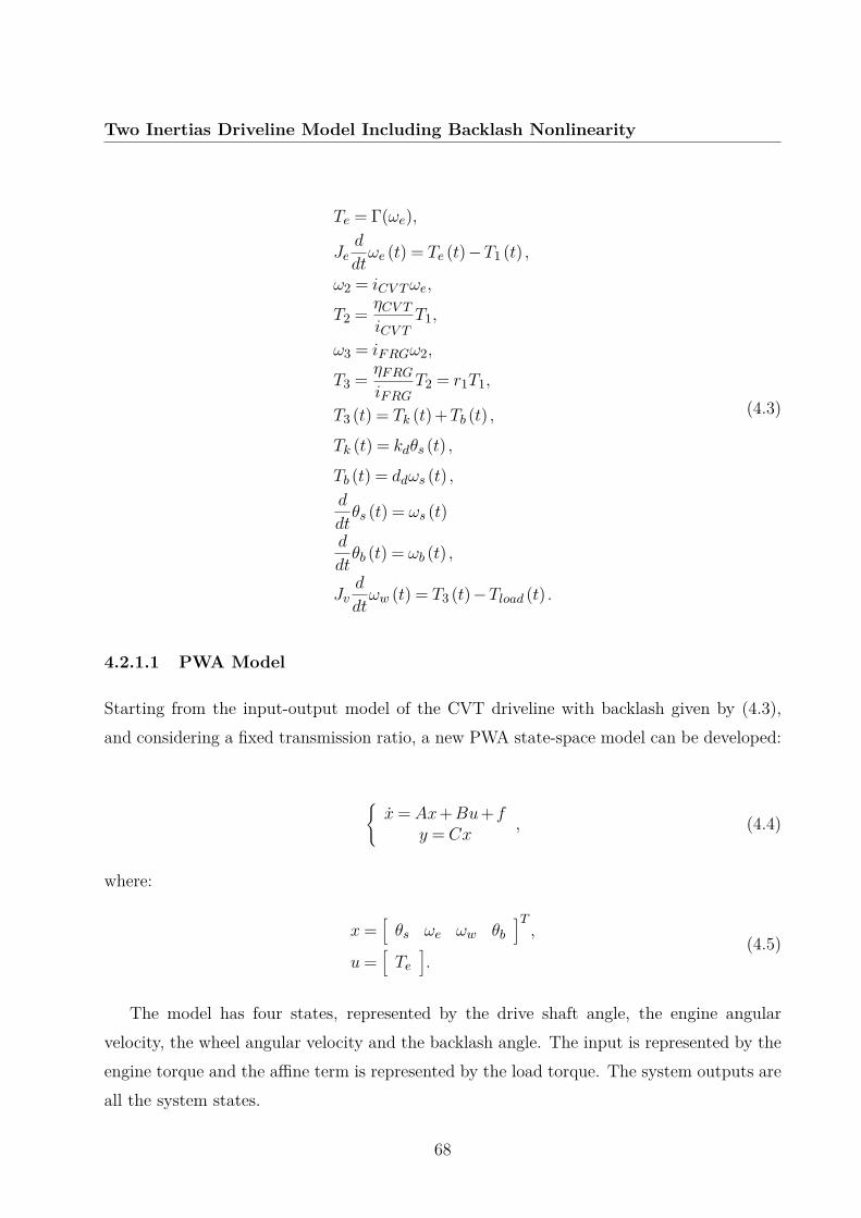
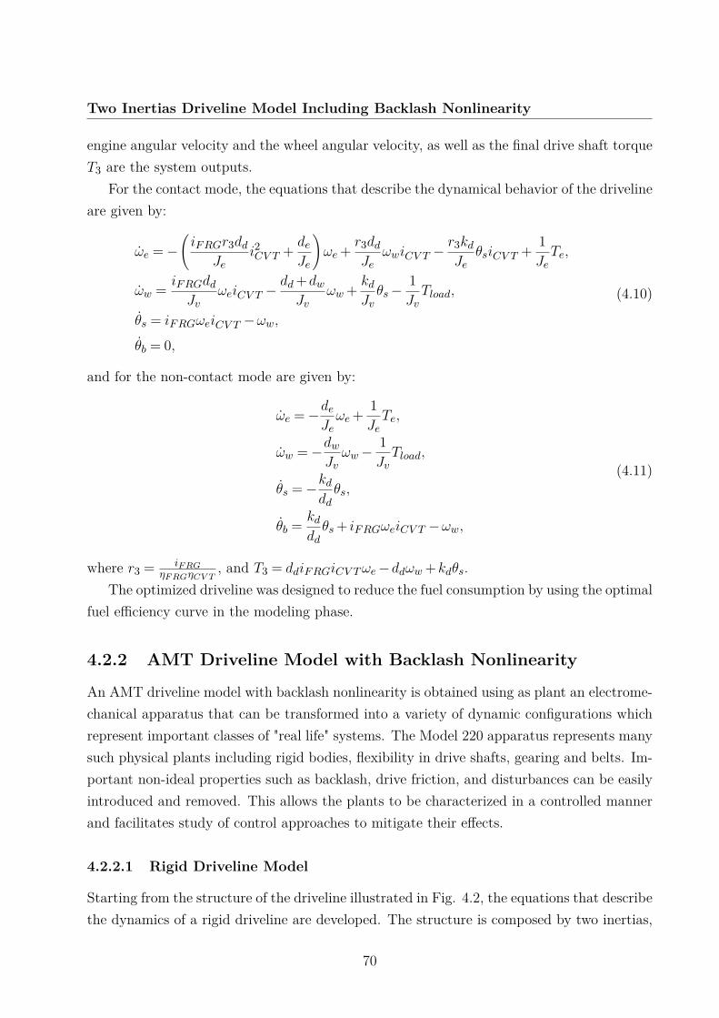
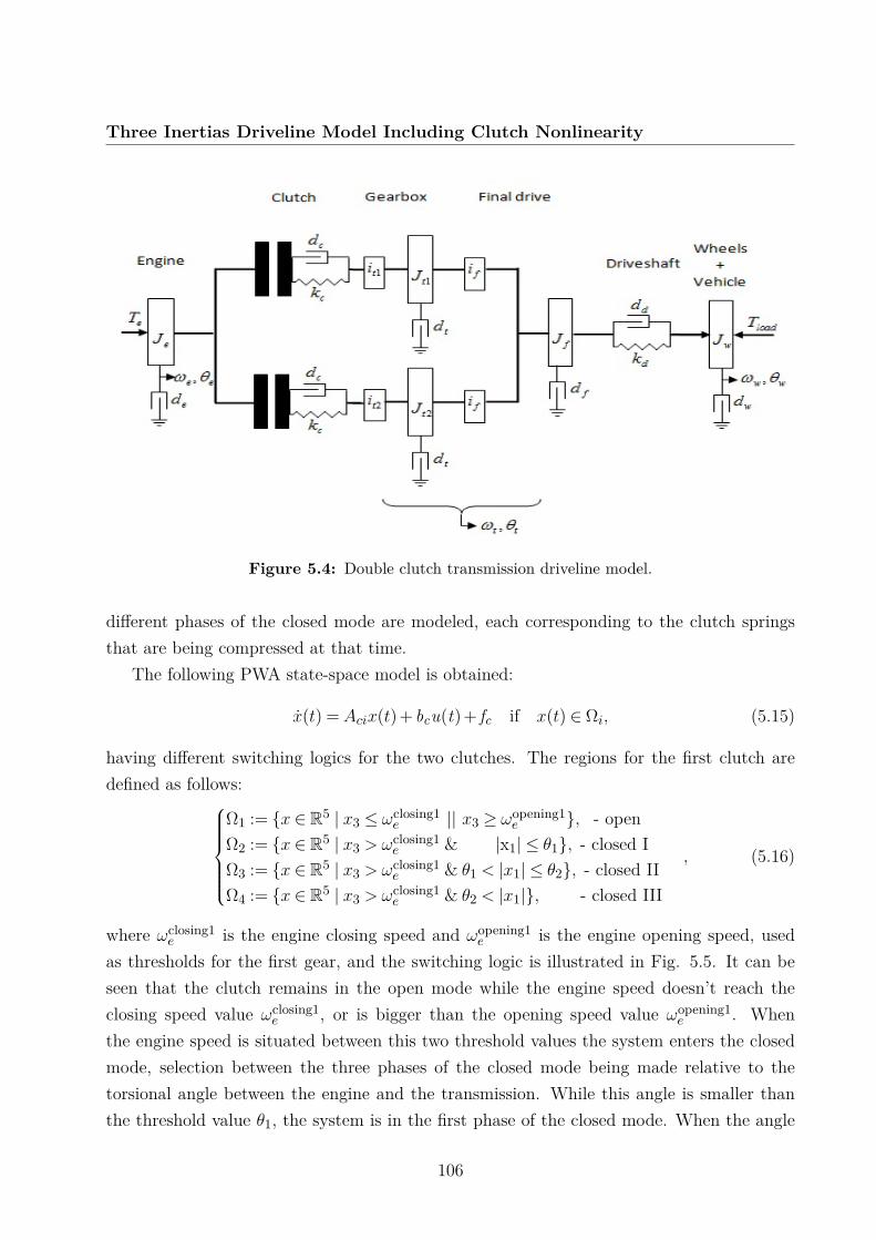
Recent studies in automotive engineering explore various engine, transmission and chassismodels and advanced control methods in order to increase overall vehicle performance, fueleconomy, safety and comfort. The goal of this thesis is overall powertrain modeling andcontrol, based on driveline subsystem integration. More complex driveline and drivelinesubsystems models are proposed, and different problems as nonlinearities introduced bybacklash and clutch are addressed, in order to improve vehicle performances.
1.1 Literature Review
An automotive powertrain is a system that includes the mechanical components which havethe function of transmitting the engine torque to the driving wheels. In order to transmitthis torque in an efficient way, a proper model of the driveline is needed for controller designpurposes, with the aim of lowering emissions, reducing fuel consumption and increasingcomfort.
1.1.1 Driveline Modeling and Control
The automotive driveline is an essential part of the vehicle and its dynamics have beenmodeled differently, according to the driving necessities. The complexity of the numerousmodels reported in the literature varies (Hrovat et al., 2000), but the two masses models aremore commonly used, and this fact is justified in (Pettersson et al., 1997), where it is shownthat this model is able to capture the first torsional vibrational mode. There are also morecomplex three-masses models reported in different research papers, as it will be indicatednext. In (Templin and Egardt, 2009) a simple driveline model with two inertias, one for theengine and the transmission, and one for the wheel and the vehicle mass, was presented.
1
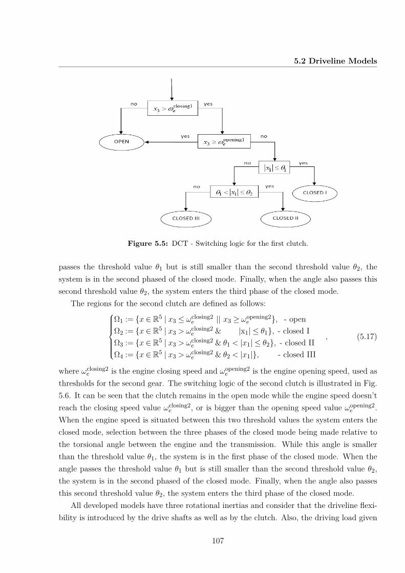
Introduction
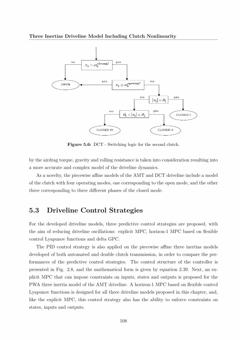
A more complex two-masses model, including a nonlinearity introduced by the backlash,was presented in (Templin, 2008). A mathematical model of a driveline was introduced in(Baumann et al., 2006) and (Bruce et al., 2005) in the form of a third order linear state-spacemodel. A simple model with the pressure in the engine manifold and the engine speed as statevariables and the throttle valve angle as control input was presented in (Saerens et al., 2008).Other two-masses model, with one inertia representing the engine and the other inertia rep-resenting the vehicle (including the clutch, main-shaft and the powertrain), were presented in(Bemporad et al., 2001), (Serrarens et al., 2004), (Larouci et al., 2007), (Song et al., 2010),(Glielmo and Vasca, 2000), (Peterson et al., 2003), (Gao et al., 2009). Two-masses mod-els for automotive driveline with continuous variable transmission (CVT) are presented in(Shen et al., 2001), (Serrarens et al., 2003) and (Liu and Yao, 2008). (Rostalski et al., 2007)presents a piecewise affine (PWA) two masses model for a driveline including a back-lash nonlinearity. In (Grotjahn et al., 2006) a two masses model was presented, with thedriveline main flexibility represented by the drive shafts, as well as a three mass modelto reproduce the behavior of a vehicle with a dual-mass flywheel. Linear and nonlinearthree masses models, in which the clutch flexibility was also considered, were presentedin (Kiencke and Nielsen, 2005). Complex three masses models that includes certain non-linear aspects of the clutch were presented in (Dolcini et al., 2005), (Glielmo et al., 2004),(Liu et al., 2011), (Garafalo et al., 2001), (Crowther et al., 2004), (Lucente et al., 2005),(Van Der Heijden et al., 2007), (Glielmo et al., 2006).
Concerning the control strategy, different approaches have also been proposed in litera-ture. In (Templin and Egardt, 2009) a linear quadratic regulator (LQR) design that dampsdriveline oscillations by compensating the driver’s engine torque demand was presented. Theperformance cost uses a weighting of the time derivative of the drive shaft torque and the dif-ference between the driver’s torque demand and the actual controller torque demand. LQRcontrollers were also proposed in (David and Natarajan, 2005) and (Dolcini, 2007). Otherlinear quadratic Gaussian controllers designed with loop transfer recovery were presented in(Pettersson et al., 1997),(Fredriksson et al., 2002),(Berriri et al., 2007), (Berriri et al., 2008).Furthermore, (Bruce et al., 2005) proposed the usage of a feed-forward controller in combi-nation with a LQR controller and considering the engine as an actuator to damp power-train oscillations. A robust pole placement strategy was employed in (Richard et al., 1999),(Stewart et al., 2005), (Stewart and Fleming, 2004), an H∞ optimization approach was pre-sented in (Lefebvre et al., 2003), while model predictive control (MPC) strategies were pro-posed in (Lagerberg and Egardt, 2005), (Rostalski et al., 2007), (Baumann et al., 2006),(Falcone et al., 2007). A feedback controller combined with a feed-forward controller is pre-sented in (Adachi et al., 2004) and (Gao et al., 2010) In (Baumann et al., 2006), a model-
2
1.1 Literature Review
based approach for anti-jerk control of passenger cars that minimizes driveline oscillationswhile retaining fast acceleration was introduced. The controller was designed with thehelp of the root locus method and an analogy to a classical PI-controller was drawn. In(Rostalski et al., 2007), a constraint was imposed on the difference between the motor speedand the load speed to minimize the driveline oscillations, while reducing the impact offorces between the mechanical parts. A clutch engagement controller based on fuzzy logicis presented in (Wu et al., 2009) a driveline control with torque observer is proposed in(Kim and Choi, 2010).
In order to improve vehicle overall performances, problems as nonlinearities introducedby backlash and clutch system are modeled, and different control strategies are proposed.
1.1.1.1 Backlash Nonlinearity
Backlash is a common problem in powertrain control because it introduces a hard nonlin-earity in the control loop for torque generation and distribution. This phenomenon occurswhenever there is a gap in the transmission link which leads to zero torque transmittedthrough the shaft to the wheels. When the backlash gap is traversed the impact results ina large shaft torque and sudden acceleration of the vehicle. Engine control systems mustcompensate for the backlash with the goal of traversing the backlash as fast as possible.
In an automotive powertrain, backlash and shaft flexibility results in an angular positiondifference between wheels and engine. The modeling of mechanical systems with backlashnonlinearities is a topic of increasing interest (Lagerberg and Egardt, 2005), (Templin, 2008),(Rostalski et al., 2007), because a backlash can lead to reduced performances and can evendestabilize the control system. Also, it can have as consequence low components reliabilityand shunt and shuffle. In order to model the mechanical system with backlash, two dif-ferent operational modes must be distinguished: backlash mode (when the two mechanicalcomponents are not in contact) and contact mode (when there is a contact between the twomechanical components resulting in a moment transmission).
New driveline management application and high-powered engines increase the need forstrategies on how to apply the engine torque in an optimal way. (Lagerberg and Egardt, 2002)presents two controllers for a powertrain model including backlash: a standard PID con-troller and a modified switching controller. The concept of PID controller with torquecompensator is presented in (Nakayama et al., 2000) for the backlash. A simple activeswitching controller for a powertrain model including backlash nonlinearities is proposed in(Tao, 1999). In (Setlur et al., 2003) a nonlinear adaptive back-stepping controller is designedin order to ensure asymptotic wheel speed and gear ratio tracking. A nonlinear predictivecontroller is designed in (Saerens et al., 2008) in order to minimize the fuel consumption
3
Introduction
and to lower emissions. A power management decoupling control strategy is presented in(Barbarisi et al., 2005) with the aim of minimizing fuel consumption and increasing drive-ability. A rule based supervisory control algorithm is designed in (Rotenberg et al., 2008)in order to improve fuel economy. A nonlinear quantitative feedback theory is applied in(Abass and Shenton, 2010), in order to control an automotive driveline with backlash non-linearity.
1.1.1.2 Clutch Nonlinearity
In recent years, the use of control systems for automated clutch and transmission actuationhas been constantly increasing, the trend towards higher levels of comfort and driving dy-namics while at the same time minimizing fuel consumption representing a major challenge.
The basic function of any type of automotive transmission is to transfer the engine torqueto the vehicle with the desired ratio smoothly and efficiently, and the most common controldevices inside the transmission are clutches and actuators. Such clutches can be hydraulicactuated, motor driven or actuated using other means.
During the last years, the automated actuated clutch systems and different valve typesused as actuators have been actively researched and different models and control strategieshave been developed: physics-based nonlinear model for an exhausting valve (Ma et al., 2008),nonlinear physical model for programmable valves (Liu and Yao, 2008), nonlinear state-space model description of the actuator that is derived based on physical principles andparameter identification (Wang et al., 2002), (Peterson et al., 2003), (Gennaro et al., 2007),(Nemeth, 2004), mathematical model obtained using identification methods for a valve ac-tuation system of an electro-hydraulic engine (Liao et al., 2008), a model for an electro-hydraulic valve used as actuator for a wet clutch (Morselli and Zanasi, 2006), dynamic mod-eling and control of electro-hydraulic wet clutches (Morselli et al., 2003), PID control for awet plate clutch actuated by a pressure reducing valve (Edelaar, 1997), predictive and piece-wise LQ control of a dry clutch engagement (Van Der Heijden et al., 2007), switched controlof an electro-pneumatic clutch actuator (Langjord et al., 2008), Model Predictive Controlof a two stage actuation system using piezoelectric actuators for controllable industrial andautomotive brakes and clutches (Neelakantan, 2008).
1.2 Outline of the Thesis
The reminder of this thesis is structured as follows.Chapter 2, entitled Driveline modeling and control presents different driveline models
and control strategies found in the literature. First, an electro-hydraulic valve-clutch system
4
1.2 Outline of the Thesis
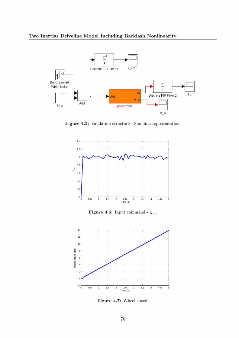
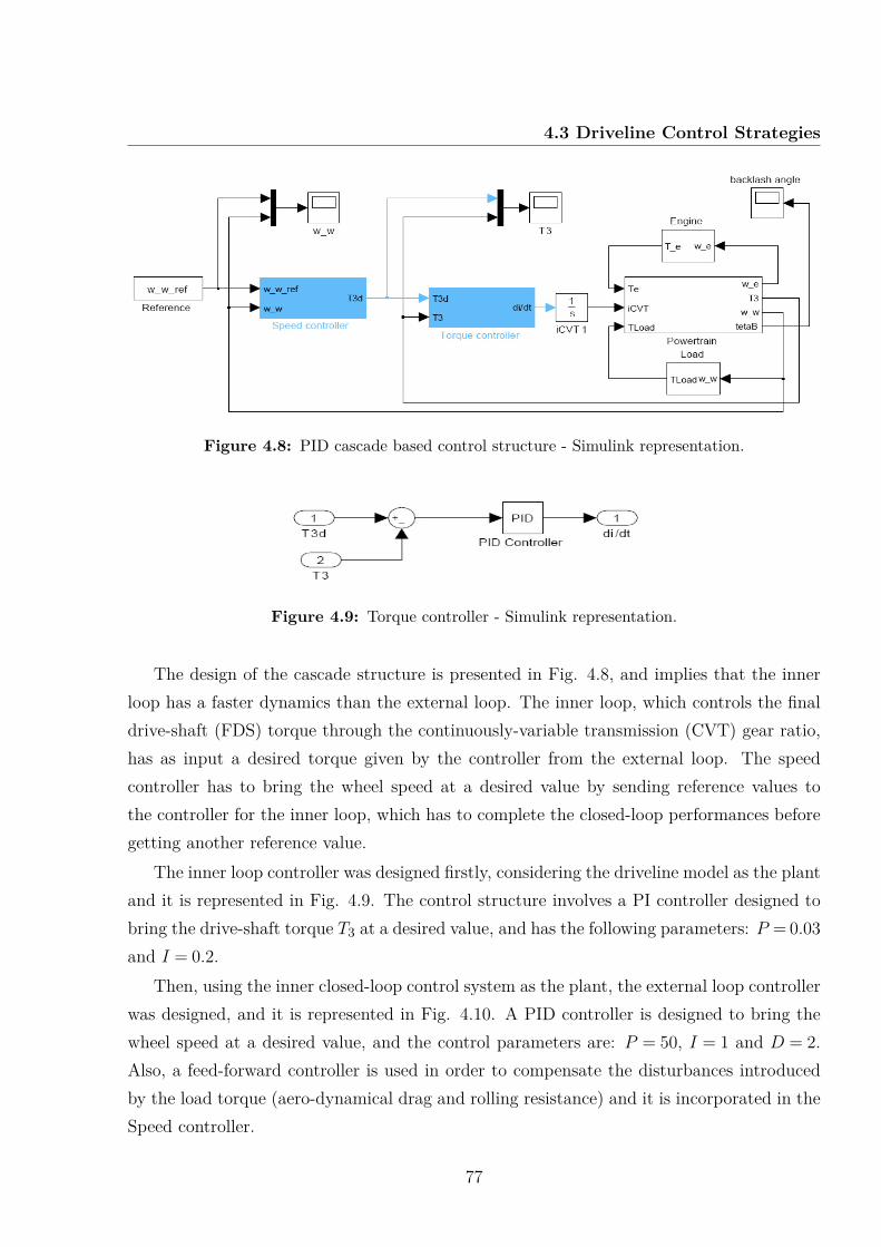
is presented, followed by three driveline models: a drive shaft model, a flexible clutch anddrive shaft model, and a continuous variable transmission drive shaft model. Next, a PID,a PID cascade based, an explicit MPC and a horizon-1 MPC based on flexible controlLyapunov function are presented as driveline control strategies. Starting from these models,in what follows, more complex driveline models are developed and also the control strategiespresented in this chapter are applied in order to obtain new controllers able to improveoverall vehicle performances.
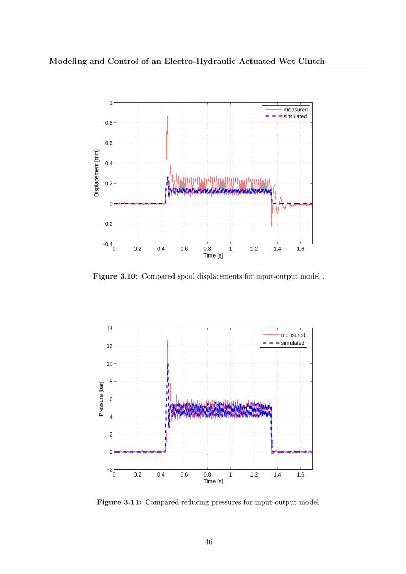
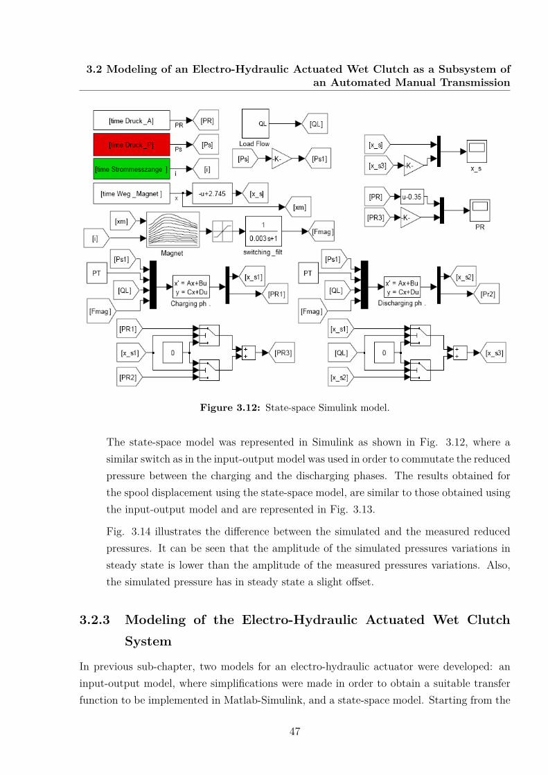
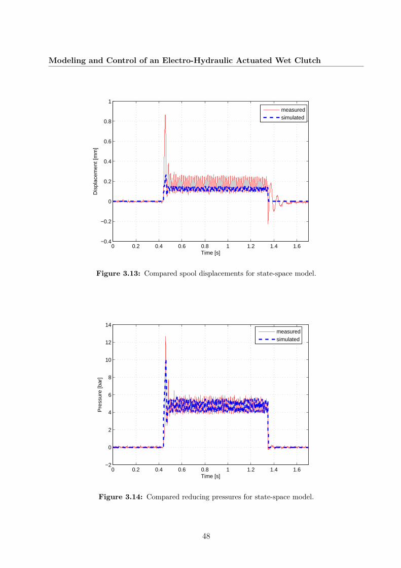
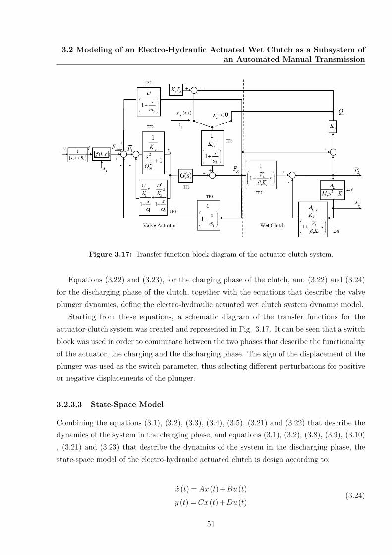
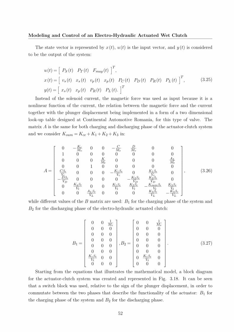
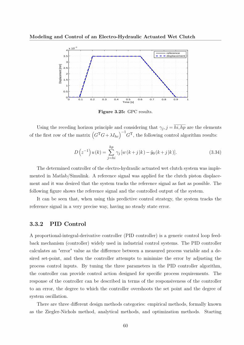
Chapter 3 is entitled Modeling and control of an electro-hydraulic actuated wet clutch.In this chapter, different models for an electro-hydraulic actuated wet clutch system in theautomatic transmission are presented. First, an input-output and a state-space model ofan electro-hydraulic pressure reducing valve are developed and stating from these, an input-output and a state space model of an electro-hydraulic actuated wet clutch is obtained.Simulators for the wet clutch and its actuator were developed and were validated with dataprovided from experiments with the real valve actuator and the clutch on a test bench. Thetest bench was provided by Continental Automotive Romania and it includes the VolkswagenDQ250 wet clutch actuated by the electro-hydraulic valve DQ500. Also, different controlstrategies are applied on the developed models and simulation result are being discussed: aGPC and a PID controller are designed in order to control the output of the electro-hydraulicactuated clutch system, the clutch piston displacement.
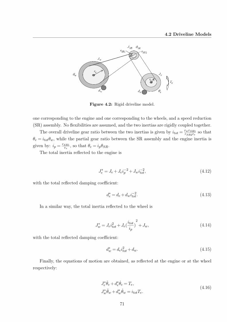
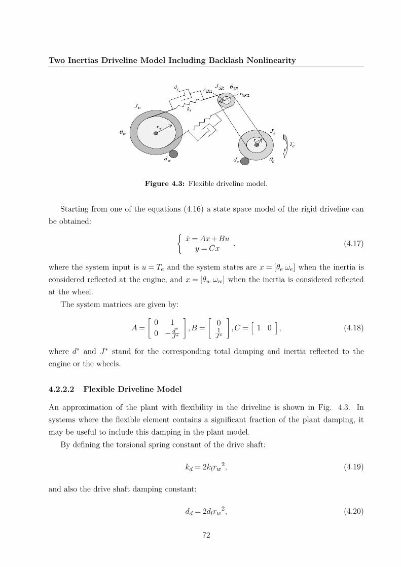
Chapter 4 is entitled Two inertias driveline model including backlash nonlinearity. Inthis chapter, different models for automotive driveline including backlash nonlinearity areproposed. First, a piecewise affine and a nonlinear state-space model for a ContinuousVariable Transmission (CVT) driveline with backlash are proposed. Simulators are developedin Matlab/Simulink for the two driveline models and different control strategies are applied.A horizon-1 MPC controller is designed for the linear model, while a PID cascade basedcontroller is applied for the nonlinear model designed to reduce the fuel consumption by usingthe optimal fuel efficiency curve in the modeling phase. Next, three models are presented foran Automated Manual Transmission (AMT) driveline based on the Industrial plant emulatorM220 : a rigid driveline model, a flexible driveline model and a flexible driveline modelincluding also backlash nonlinearity. Then, real time experiments are conducted on thepresented models in order to test the influences given by drive shaft flexibility and backlashangle, while applying a horizon-1 MPC controller.
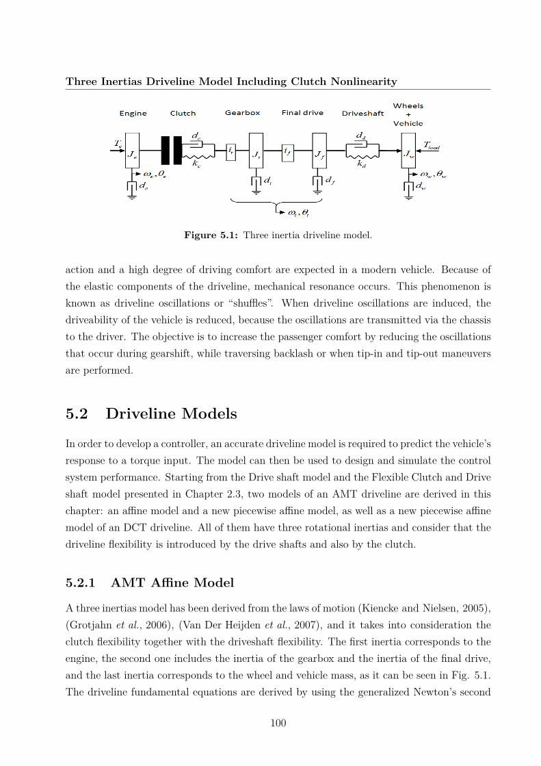
Chapter 5 is entitled Three inertias driveline model including clutch nonlinearity. Thischapter deals with the problem of damping driveline oscillations in order to improve passen-ger comfort. Three driveline models with three inertias are proposed: a state-space affinemodel and a new state-space piecewise affine model of an automated manual transmission
5
Introduction
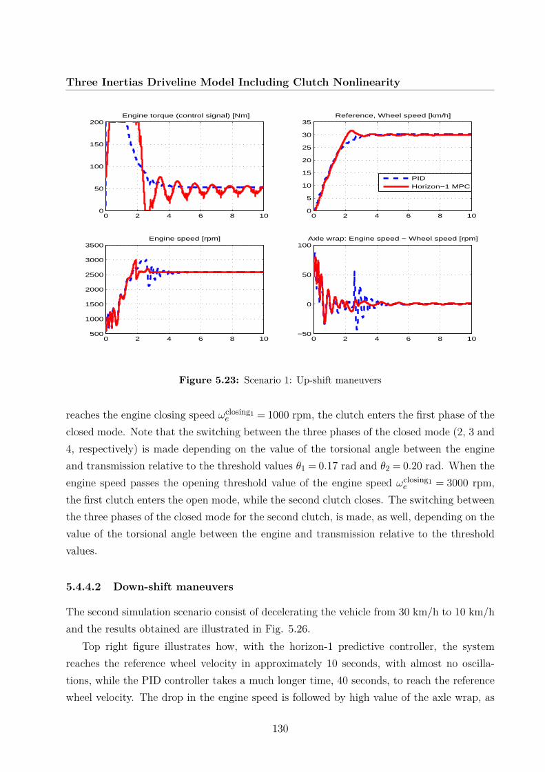
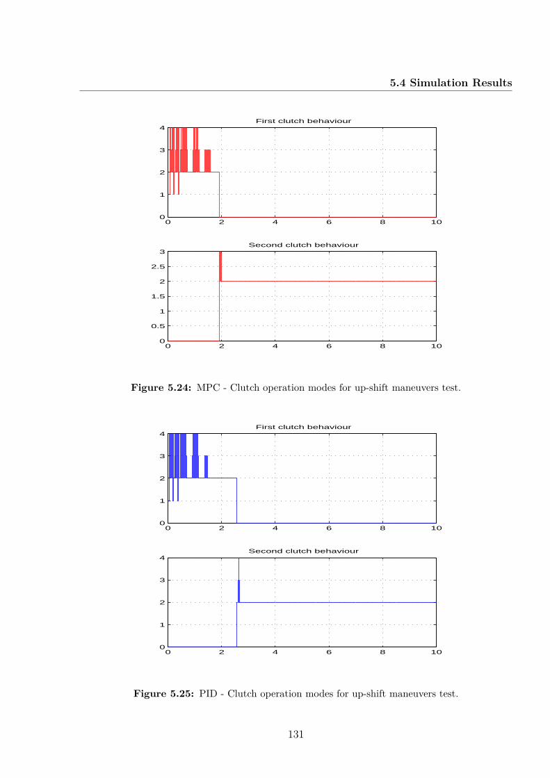
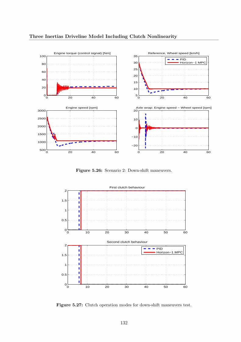
(AMT) driveline, and a new state-space piecewise affine model of a double clutch trans-mission (DCT) driveline, all of them taking into consideration the drive shafts as well asthe clutch flexibilities. Three controllers are implemented for the developed models: ex-plicit MPC, delta GPC and horizon-1 MPC, and the experiments showed that the horizon-1MPC control scheme can handle both the performance/physical constraints and the strictlimitations on the computational complexity corresponding to vehicle driveline oscillationsdamping.
1.3 List of Publications
This thesis is based on fourteen published articles, divided as follows: one ISI indexed paper(IF=1.762), one Zentralblatt Math indexed paper, three ISI Proceedings papers, four IEEEconference papers, two IFAC conference papers and three papers published at internationalconferences where paper review is conducted.
Chapter 3 contains results published in:
• (Balau et al., 2009a) A. E. Balau, C. F. Caruntu, D. I. Patrascu, C. Lazar, M. H.Matcovschi and O. Pastravanu. Modeling of a Pressure Reducing Valve Actuator forAutomotive Applications. In 18th IEEE International Conference on Control Applica-tions, Part of 2009 IEEE Multi-conference on Systems and Control, Saint Petersburg,Russia, 2009.
• (Balau et al., 2009b) A. E. Balau, C. F. Caruntu, C. Lazar and D. I. Patrascu. NewModel for Predictive Control of an Electro-Hydraulic Actuated Clutch. In The 18thInternational Conference on FUEL ECONOMY, SAFETY and RELIABILITY of MO-TOR VEHICLES (ESFA 2009), Bucharest, Romania, 2009.
• (Patrascu, Balau et al., 2009) D. I. Patrascu, A. E. Balau, C. F. Caruntu, C. Lazar,M. H. Matcovschi and O. Pastravanu. Modelling of a Solenoid Valve Actuator forAutomotive Control Systems. In The 1tth International Conference on Control Systemsand Computer Science, Bucharest, Romania, 2009.
• (Caruntu, Matcovschi, Balau et al., 2009) C. F. Caruntu, M. H. Matcovschi, A. E.Balau, D. I. Patrascu, C. Lazar and O. Pastravanu. Modelling of An ElectromagneticValve Actuator. Buletinul Institutului Politehnic din Iasi, vol. Tome LV (LIX), Fasc.2, pages 9–28, 2009.
6
1.3 List of Publications
• (Balau et al., 2010) A. E. Balau, C. F. Caruntu and C. Lazar. State-space model of anelectro-hydraulic actuated wet clutch. In IFAC Symposium Advances in AutomotiveControl, Munchen, Germany, 2010.
• (Balau et al., 2011a) A. E. Balau, C. F. Caruntu and C. Lazar. Simulation and Controlof an Electro-Hydraulic Actuated Clutch. Mechanical Systems and Signal Processing,vol. 25, pages 1911–1922, 2011.
• (C.Lazar, Caruntu and Balau, 2010) C. Lazar, C. F. Caruntu and A. E. Balau. Mod-elling and Predictive Control of an Electro-Hydraulic Actuated Wet Clutch for Auto-matic Transmission. In IEEE Symposium on Industrial Electronics, Bari, Italy, 2010.
• (Caruntu, Balau and C.Lazar, 2010a) C. F. Caruntu, A. E. Balau and C. Lazar. Net-worked Predictive Control Strategy for an Electro-Hydraulic Actuated Wet Clutch. InIFAC Symposium Advances in Automotive Control, Munchen, Germany, 2010.
• (Balau and C.Lazar, 2011a) A. E. Balau and C. Lazar. Predictive control of an electro-hydraulic actuated wet clutch. In The 15th International Conference on System Theory,Control and Computing, Sinaia, Romania, 2011.
Chapter 4 contains results published in:
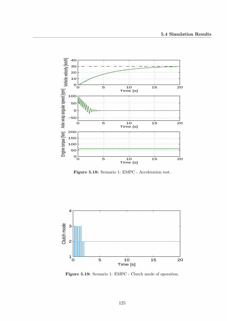
• (Caruntu, Balau and C.Lazar, 2010b) C. F. Caruntu, A. E. Balau and C. Lazar. Cas-cade based Control of a Drivetrain with Backlash. In 12th International Conference onOptimization of Electrical and Electronic Equipment, Brasov, Romania, 2010.
Chapter 5 contains results published in:
• (Balau et al., 2011b) A. E. Balau, C. F. Caruntu and C. Lazar. Driveline oscillationsmodeling and control. In The 18th International Conference on Control Systems andComputer Science, Bucharest, Romania, 2011.
• (Balau and C.Lazar, 2011b) A.E. Balau and C. Lazar. One Step Ahead MPC for anAutomotive Control Application. In The 2nd Eastern European Regional Conferenceon the Engineering of Computer Based Systems, Bratislava, Slovakia, 2011.
• (Caruntu, Balau et al., 2011) C. F. Caruntu, A. E. Balau, M. Lazar, P. P. J. v. d. Boshand S. Di Cairano. A predictive control solution for driveline oscillations damping. InThe 14th International Conference on Hybrid Systems: Computation and Control,Chicago, USA, 2011.
7
Introduction
• (Halauca, Balau and C.Lazar, 2011) C. Halauca, A. E. Balau and C. Lazar. StateSpace Delta GPC for Automotive Powertrain Systems. In The16th IEEE InternationalConference on Emerging Technologies and Factory Automation, 2011.
8
Chapter 2
Driveline Modeling and Control
An automotive powertrain is a system that includes the mechanical components which havethe function of transmitting the engine torque to the driving wheels. In order to transmitthis torque in an efficient way, a proper model of the driveline is needed for controllerdesign purposes with the aim of lowering emissions, reducing fuel consumption and increasingcomfort. Recent studies in automotive engineering explore various engine, transmission andchassis models and advanced control methods in order to increase overall vehicle performance.
2.1 Introduction
The driveline is a fundamental part of a vehicle and its dynamics have been modeled indifferent ways, according to the purpose. The aim of the modeling is to find the mostsignificant physical effects that have as negative result oscillations in the wheel speed. Mostexperiments consider in the modeling phase low gears because the higher torque transmittedto the drive shaft is obtained in the lower gear. Also, the amplitudes of the resonances in thewheel speed are higher for lower gears, because the load and vehicle mass appear reducedby the high conversion ratio.
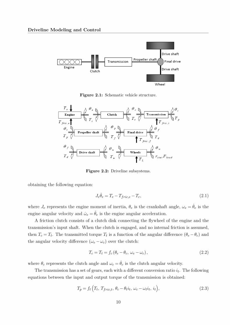
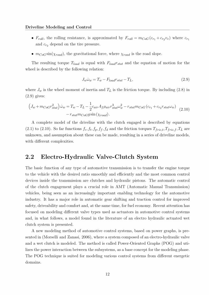
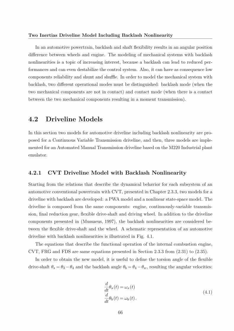
The structure of a passenger car consists, in general, of the following parts: engine, clutch,transmission, propeller shaft, final drive, drive shafts and wheels, as it can be seen in Fig. 2.1.In what follows, the fundamental equations of the driveline will be derived by using the gen-eralized Newton’s second law of motion, as described in (Kiencke and Nielsen, 2005). FigureFig. 2.2 shows the labels, the inputs and the outputs of each subsystem of the considereddriveline, and relations between them will be described for each part.
The output engine torque is given by the driving engine torque Te resulted from thecombustion, the internal engine friction Tfric,e, and the external load from the clutch Tc,
9
Driveline Modeling and Control
Figure 2.1: Schematic vehicle structure.
Figure 2.2: Driveline subsystems.
obtaining the following equation:
Jeθe = Te−Tfric,e−Tc, (2.1)
where Je represents the engine moment of inertia, θe is the crankshaft angle, ωe = θe is theengine angular velocity and ωe = θe is the engine angular acceleration.
A friction clutch consists of a clutch disk connecting the flywheel of the engine and thetransmission’s input shaft. When the clutch is engaged, and no internal friction is assumed,then Tc = Tt. The transmitted torque Tt is a function of the angular difference (θe−θc) andthe angular velocity difference (ωe−ωc) over the clutch:
Tc = Tt = fc (θe− θc, ωe−ωc) , (2.2)
where θc represents the clutch angle and ωc = θc is the clutch angular velocity.The transmission has a set of gears, each with a different conversion ratio it. The following
equations between the input and output torque of the transmission is obtained:
Tp = ft(Tt, Tfric,t, θc− θtit, ωc−ωtit, it
), (2.3)
10
2.1 Introduction
where Tp is the propeller shaft torque, Tfric,t is the internal friction torque of the trans-mission, θt is the transmission angle and ωt = θt is the corresponding angular velocity. Thereason for considering the angle difference θc−θtit is the possibility of having torsional effectsin the transmission.
The propeller shaft connects the transmission’s output shaft with the final drive. Nofriction is assumed so Tp = Tf , giving the following equation:
Tp = Tf = fp (θt− θp, ωt−ωp) , (2.4)
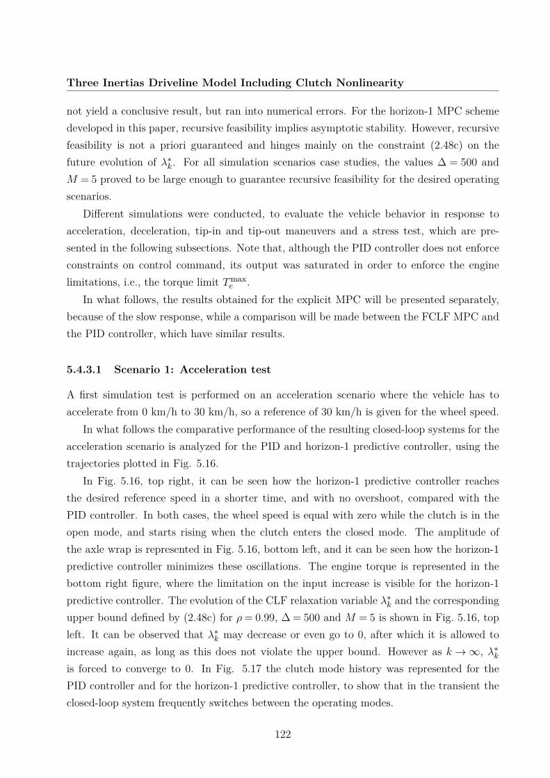
where Tf is the final drive torque, θp is the propeller shaft angle and ωp = θp is the corre-sponding angular velocity.
The final drive is characterized by a conversion ratio if in the same way as for thetransmission. The following relation between the input and the output torque holds:
Td = ff(Tf , Tfric,f , θp− θf if , ωp−ωf if , if
), (2.5)
where Tfric,f is the internal friction torque of the final drive, Td is the drive shaft torque, θfis the final drive angle and ωf = θf is the corresponding angular velocity.
The drive shafts is the subsystem that connects the wheel to the final drive. Assumingthat θw is the wheel angle, the rotational wheel velocity ωw = θw is the same for both wheelsand neglecting the vehicle dynamics, the rotational equivalent wheel velocity shall be equalto the velocity of the vehicle body’s center of gravity vv:
ωw = vvrstat
, (2.6)
where rstat represents the wheel radius. The shafts are modeled as one shaft and assumingthat no friction exists Tw = Td the following equation for the wheel torque Tw results:
Tw = Td = fd(θf − θw, ωf −ωw
). (2.7)
Newton’s second law in the longitudinal direction for a vehicle with mass mCoG andspeed vv, gives:
The load force Fload is described by the sum of following quantities:
• Fairdrag, the air drag, is approximated by Fairdrag = 12cairAfρairv
2v , where cair is the
drag coefficient, Af is the maximum vehicle cross section area and ρair is the air density.
11
Driveline Modeling and Control
• Froll, the rolling resistance, is approximated by Froll = mCoG (cr1 + cr2vv) where cr1
and cr2 depend on the tire pressure.
• mCoG sin(χroad), the gravitational force, where χroad is the road slope.
The resulting torque Tload is equal with Floadrstat and the equation of motion for thewheel is described by the following relation:
Jwωw = Tw−Floadrstat−TL, (2.9)
where Jw is the wheel moment of inertia and TL is the friction torque. By including (2.8) in(2.9) gives:(Jw +mCoGr
2stat
)ωw = Tw−TL−
12cairAfρairr
3statω
2w− rstatmCoG (cr1 + cr2rstatωw)
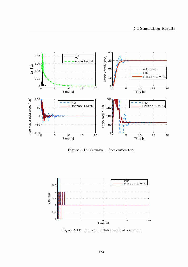
− rstatmCoGg sin(χroad) .(2.10)
A complete model of the driveline with the clutch engaged is described by equations(2.1) to (2.10). So far functions fc,ft,fp,ff ,fd and the friction torques Tfric,t,Tfric,f ,TL areunknown, and assumption about these can be made, resulting in a series of driveline models,with different complexities.
2.2 Electro-Hydraulic Valve-Clutch System
The basic function of any type of automotive transmission is to transfer the engine torqueto the vehicle with the desired ratio smoothly and efficiently and the most common controldevices inside the transmission are clutches and hydraulic pistons. The automatic controlof the clutch engagement plays a crucial role in AMT (Automatic Manual Transmission)vehicles, being seen as an increasingly important enabling technology for the automotiveindustry. It has a major role in automatic gear shifting and traction control for improvedsafety, driveability and comfort and, at the same time, for fuel economy. Recent attention hasfocused on modeling different valve types used as actuators in automotive control systemsand, in what follows, a model found in the literature of an electro hydraulic actuated wetclutch system is presented.
A new modeling method of automotive control systems, based on power graphs, is pre-sented in (Morselli and Zanasi, 2006), where a system composed of an electro-hydraulic valveand a wet clutch is modeled. The method is called Power-Oriented Graphs (POG) and uti-lizes the power interaction between the subsystems, as a base concept for the modeling phase.The POG technique is suited for modeling various control systems from different energeticdomains.
12
2.2 Electro-Hydraulic Valve-Clutch System
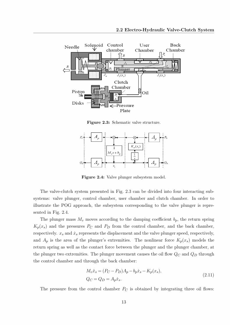
Figure 2.3: Schematic valve structure.
Figure 2.4: Valve plunger subsystem model.
The valve-clutch system presented in Fig. 2.3 can be divided into four interacting sub-systems: valve plunger, control chamber, user chamber and clutch chamber. In order toillustrate the POG approach, the subsystem corresponding to the valve plunger is repre-sented in Fig. 2.4.
The plunger mass Mv moves according to the damping coefficient bp, the return springKp(xs) and the pressures PC and PD from the control chamber, and the back chamber,respectively. xs and xs represents the displacement and the valve plunger speed, respectively,and Ap is the area of the plunger’s extremities. The nonlinear force Kp(xs) models thereturn spring as well as the contact force between the plunger and the plunger chamber, atthe plunger two extremities. The plunger movement causes the oil flow QC and QD throughthe control chamber and through the back chamber:
Mvxs = (PC −PD)Ap− bpxs−Kp(xs),
QC =QD = Apxs.(2.11)
The pressure from the control chamber PC is obtained by integrating three oil flows:
13
Driveline Modeling and Control
the flow Q5 from the power source Ps, the flow QC due to the plunger movement, and theflow Qw through the variable discharging orifice. The very small hydraulic capacity CC
stores potential energy in terms of oil pressure and it takes into account the small elasticdeformation of the valve case and the oil stiffness:
CC PC =Q5−QC −Qw. (2.12)
Depending on the plunger position, the output user chamber is connected either to thepower supply through the variable orifice J1 or to the oil tank by the orifice J3. Also, theuser chamber is connected to the back chamber through orifice J4. This orifice plays tworoles: it implements the feedback action since PD becomes a measure of the user pressurePR, and it has the damping effect that avoids plunger oscillations.
The back chamber and the user chamber are modeled as two small hydraulic capacities,as for the control chamber:
CDPD =QD−Q4,
CRPR =Q1 +Q4−Q3−QR.(2.13)
The user chamber is connected to the clutch chamber by means of a pipe with a dynamicthat cannot be neglected and is described by four elements: the user chamber capacityCR, the hydraulic resistance RL, the pipe hydraulic inductance LL and the clutch chambercapacity CL:
LLQR = Pl−PL = PR−PQR−PL,
PR−Pl = QR |QR|CL
=RL(QR),
CLPL =QR−ALz.
(2.14)
where PL is the clutch pressure.The motion of the pressure plate under the effects of the pressure PL, the elastic force
KM (z) and the viscous friction bf are given by the following equations:
Mpz = PLAL− bfxz−KM (z)−Kbcsgn(z),
KM (z) =KF (z) +KD(z).(2.15)
where Mp is the clutch plunger mass, AL is the clutch piston area, KF (z) represents theforce of the return springs and the contact with the gearbox at the two extreme pressureplate positions, and KD(z) is the force generated by the compression of the clutch discs thatdetermines the maximum torque through the clutch.
This combined equations model the valve-clutch system using the POG technique and thesimulations results are very similar to the experimental data, providing that the modelingapproach is suitable to automotive control systems.
14
2.3 Driveline Models
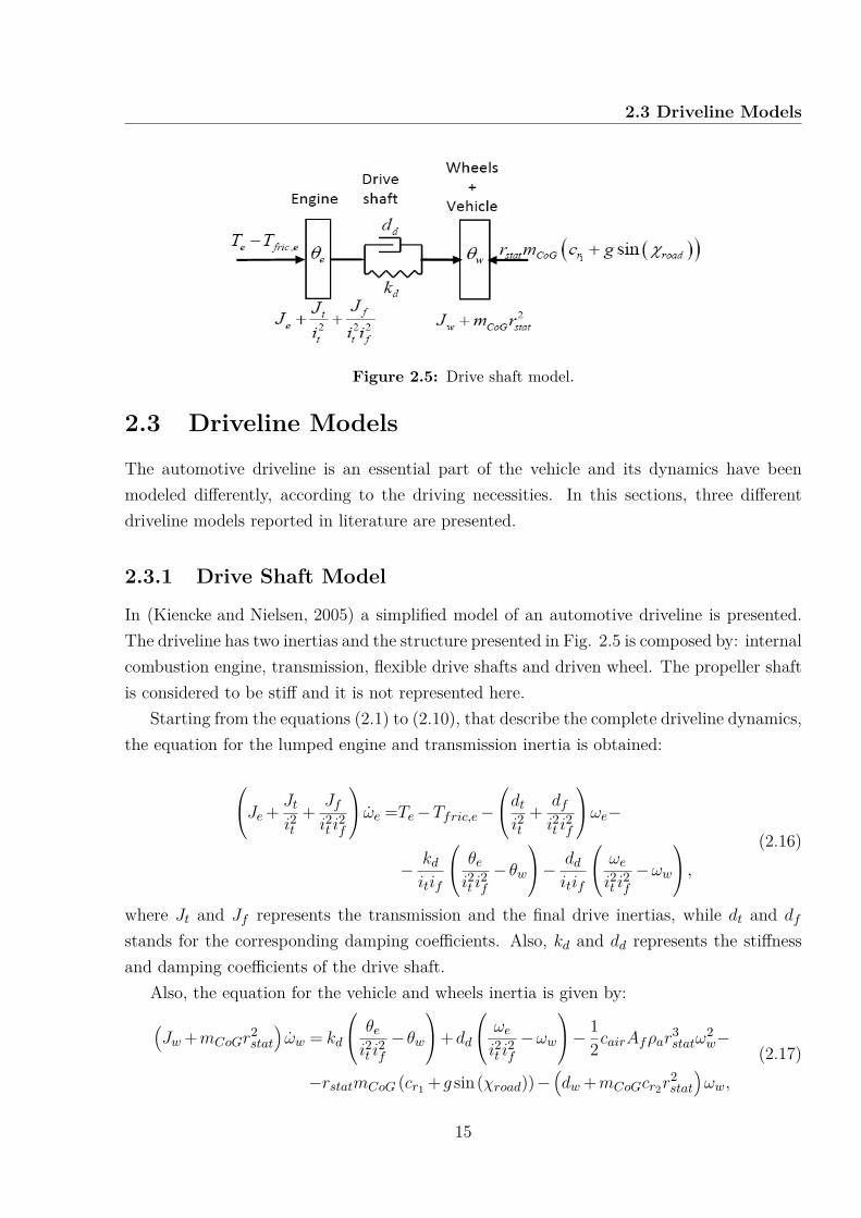
Figure 2.5: Drive shaft model.
2.3 Driveline Models
The automotive driveline is an essential part of the vehicle and its dynamics have beenmodeled differently, according to the driving necessities. In this sections, three differentdriveline models reported in literature are presented.
2.3.1 Drive Shaft Model
In (Kiencke and Nielsen, 2005) a simplified model of an automotive driveline is presented.The driveline has two inertias and the structure presented in Fig. 2.5 is composed by: internalcombustion engine, transmission, flexible drive shafts and driven wheel. The propeller shaftis considered to be stiff and it is not represented here.
Starting from the equations (2.1) to (2.10), that describe the complete driveline dynamics,the equation for the lumped engine and transmission inertia is obtained:
Je+ Jti2t
+ Jfi2t i
2f
ωe =Te−Tfric,e−dti2t
+ dfi2t i
2f
ωe−− kditif
θei2t i
2f
− θw
− dditif
ωei2t i
2f
−ωw
,(2.16)
where Jt and Jf represents the transmission and the final drive inertias, while dt and df
stands for the corresponding damping coefficients. Also, kd and dd represents the stiffnessand damping coefficients of the drive shaft.
Also, the equation for the vehicle and wheels inertia is given by:(Jw +mCoGr
2stat
)ωw = kd
θei2t i
2f
− θw
+dd
ωei2t i
2f
−ωw
− 12cairAfρar
3statω
2w−
−rstatmCoG (cr1 +g sin(χroad))−(dw +mCoGcr2r
2stat
)ωw,
(2.17)
15
Driveline Modeling and Control
where dw represents the damping coefficient of the wheel.The drive shaft model is the simplest one considered, and the drive shaft torsion, the
engine speed and the wheel speed are used as states, according to:
x1 = θeif it− θw
x2 = ωe
x3 = ωw
. (2.18)
Also, taking into consideration that:
J1 = Je+ Jti2t
+ Jfi2t i
2f
J2 = Jw +mCoGr2stat
d1 = dti2t
+ dfi2t i
2f
d2 = dw +mCoGcr2r2stat
l = rstatmCoG (cr1 +g sin(χroad))
, (2.19)
the following state-space representation is obtain:
x= Ax+Bu+Hl, (2.20)
consisting of the system matrices:
A=
0 1
if it−1
− kif itJ1
−d1+ dif it
2
J1d
if itJ1kJ2
0 dif itJ2
−d+d2J2
, (2.21)
B =
01J10
,H =
00−1J2
. (2.22)
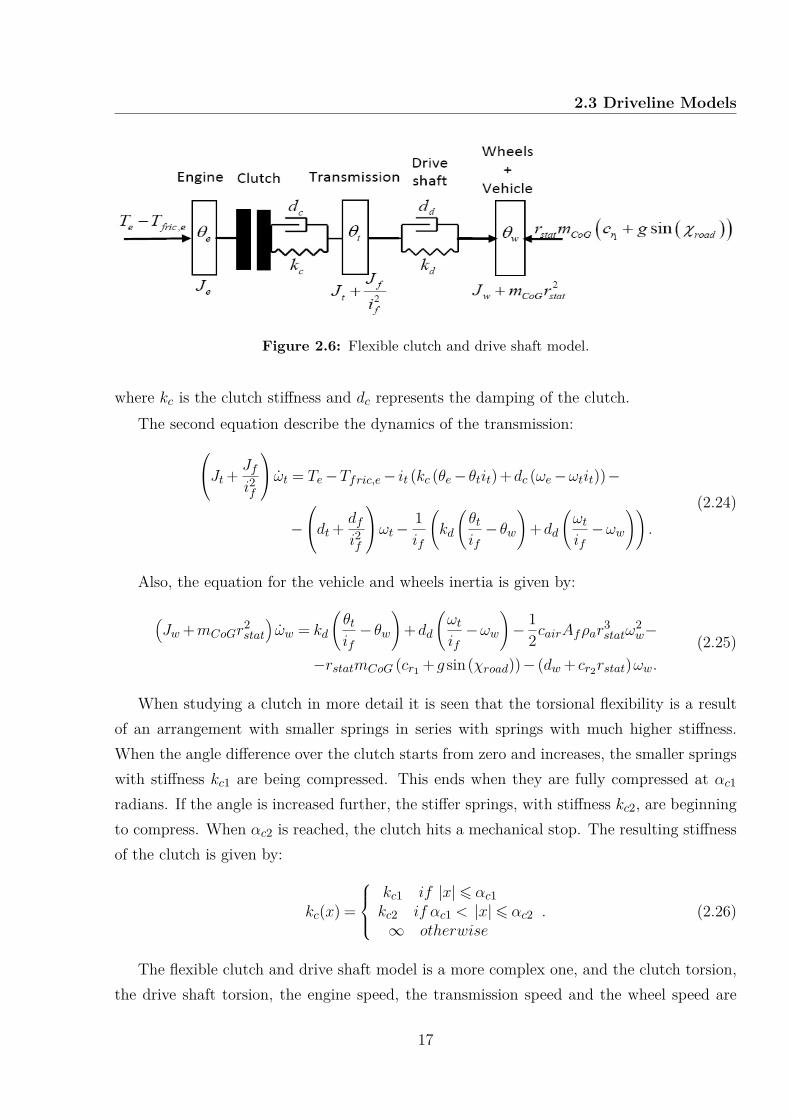
2.3.2 Flexible Clutch and Drive Shaft Model
A more complex model including two torsional flexibilities, the drive shaft and the clutchis also presented in (Kiencke and Nielsen, 2005). The driveline has three inertias like rep-resented in Fig. 2.6, one corresponding to the internal combustion engine, one for thetransmission, and one for the driven wheel.
The equation that describe the engine dynamics is given by:
When studying a clutch in more detail it is seen that the torsional flexibility is a resultof an arrangement with smaller springs in series with springs with much higher stiffness.When the angle difference over the clutch starts from zero and increases, the smaller springswith stiffness kc1 are being compressed. This ends when they are fully compressed at αc1radians. If the angle is increased further, the stiffer springs, with stiffness kc2, are beginningto compress. When αc2 is reached, the clutch hits a mechanical stop. The resulting stiffnessof the clutch is given by:
kc(x) =
kc1 if |x|6 αc1kc2 if αc1 < |x|6 αc2∞ otherwise
. (2.26)
The flexible clutch and drive shaft model is a more complex one, and the clutch torsion,the drive shaft torsion, the engine speed, the transmission speed and the wheel speed are
17
Driveline Modeling and Control
used as states, according to:
x1 = θe− θtit
x2 = θtif− θw
x3 = ωe
x4 = ωt
x5 = ωw
. (2.27)
The state-space formulation of the linear clutch and drive shaft model consist of thesystem matrices defined next:
Ac =
0 0 1 −it 00 0 0 1
if−1
− kcJ1
0 −dcJ1
dcitJ1
0
kcitJ2
− kdifJ2
dcitJ2
−dci2t +d2+ dd
i2f
J2ddifJ2
0 kdJ3
0 ddifJ3
−d3−ddJ3
, (2.28)
B =
001J100
,H =
0000−1J2
, (2.29)
where
J1 = Je
J2 = Jt+Jfi2f
J3 = Jw +mCoGr2stat
d2 = dt+dfi2f
d3 = dw +mCoGcr2r2stat
. (2.30)
2.3.3 Continuous Variable Transmission Drive Shaft Model
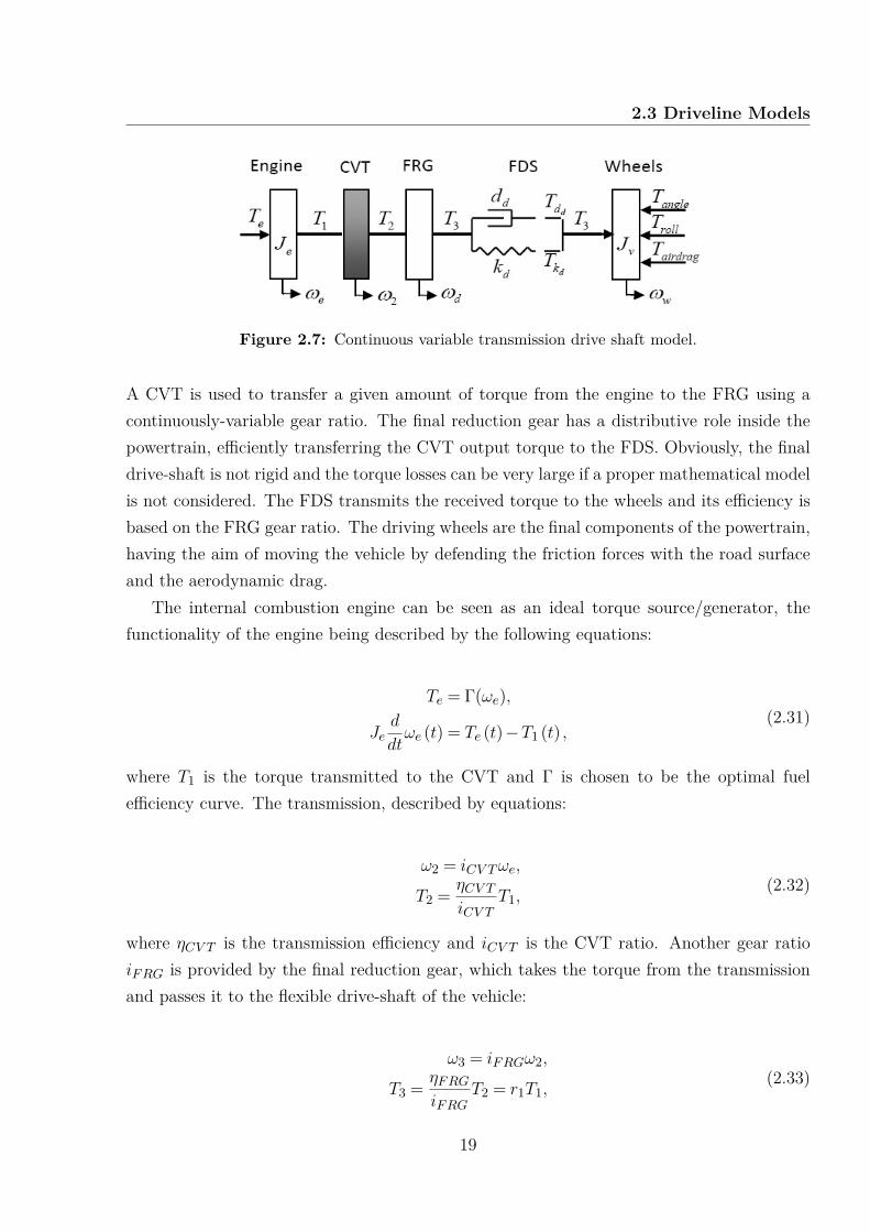
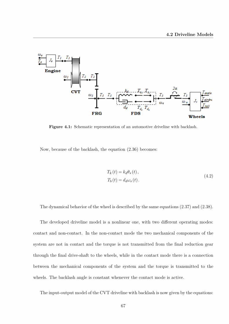
In (Mussaeus, 1997), a nonlinear model for a continuously-variable transmission driveline isdeveloped. The powertrain is represented in Fig. 2.7 and it is composed from the followingcomponents: engine, continuously-variable transmission (CVT), final reduction gear (FRG),flexible drive shaft (FDS) and driving wheel, which can be seen as input-output blocks. Theengine generates a toque which is transmitted towards the wheels through the driveline.
A CVT is used to transfer a given amount of torque from the engine to the FRG using acontinuously-variable gear ratio. The final reduction gear has a distributive role inside thepowertrain, efficiently transferring the CVT output torque to the FDS. Obviously, the finaldrive-shaft is not rigid and the torque losses can be very large if a proper mathematical modelis not considered. The FDS transmits the received torque to the wheels and its efficiency isbased on the FRG gear ratio. The driving wheels are the final components of the powertrain,having the aim of moving the vehicle by defending the friction forces with the road surfaceand the aerodynamic drag.
The internal combustion engine can be seen as an ideal torque source/generator, thefunctionality of the engine being described by the following equations:
Te = Γ(ωe),
Jed
dtωe (t) = Te (t)−T1 (t) ,
(2.31)
where T1 is the torque transmitted to the CVT and Γ is chosen to be the optimal fuelefficiency curve. The transmission, described by equations:
ω2 = iCV Tωe,
T2 = ηCV TiCV T
T1,(2.32)
where ηCV T is the transmission efficiency and iCV T is the CVT ratio. Another gear ratioiFRG is provided by the final reduction gear, which takes the torque from the transmissionand passes it to the flexible drive-shaft of the vehicle:
ω3 = iFRGω2,
T3 = ηFRGiFRG
T2 = r1T1,(2.33)
19
Driveline Modeling and Control
where r1 = ηF RGηCV TiF RGiCV T
and ηFRG is the flexible drive-shaft efficiency. Considering the flexibledrive-shaft speed related to the engine speed and solving 2.32 in 2.33 yields:
ω3 (t) = ωe (t)r2
, (2.34)
where r2 = 1iF RGiCV T
.The powertrain flexibility is given by the flexible drive-shaft, which is characterized by
an elasticity factor kd = Jvπ2 and a damping coefficient dd = 2
√kdJv, both used to calculate
the FDS torque:
T3 (t) = Tk (t) +Tb (t) , (2.35)
where we have:
Tk = kd
t∫0
(ω3−ωw)dσ,
Tb = dd (ω3−ωw) .
(2.36)
The dynamical behavior of the wheel is described by the following equation:
Jvd
dtωw (t) = T3 (t)−Tload (t) , (2.37)
where
Jv = r2statmCOG,
Tload (t) = Troll (t) +Tairdrag (t) +Tangle (t) ,
Tairdrag (t) = c1ω2w (t) ,
Troll (t) = c2mCOG,
Tangle (t) = 0.
(2.38)
The torque due to hill climbing and all other disturbances are summarized in Tangle,which is assumed to be unknown and might therefore be subject to estimation, Tairdrag isthe load torques due to aerodynamic drag and c1 and c2 are constants.
The optimized powertrain was designed to reduce the fuel consumption by using theoptimal fuel efficiency curve in the modeling phase.
20
2.4 Driveline Control Strategies
2.4 Driveline Control Strategies
Next step after developing the driveline model, is to find the proper control strategy to obtainthe desired performances. In this section, different control strategies proposed in literaturefor improving overall performances are presented.
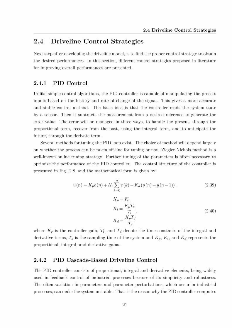
2.4.1 PID Control
Unlike simple control algorithms, the PID controller is capable of manipulating the processinputs based on the history and rate of change of the signal. This gives a more accurateand stable control method. The basic idea is that the controller reads the system stateby a sensor. Then it subtracts the measurement from a desired reference to generate theerror value. The error will be managed in three ways, to handle the present, through theproportional term, recover from the past, using the integral term, and to anticipate thefuture, through the derivate term.
Several methods for tuning the PID loop exist. The choice of method will depend largelyon whether the process can be taken off-line for tuning or not. Ziegler-Nichols method is awell-known online tuning strategy. Further tuning of the parameters is often necessary tooptimize the performance of the PID controller. The control structure of the controller ispresented in Fig. 2.8, and the mathematical form is given by:
u(n) =Kpe(n) +Ki
n∑k=0
e(k)−Kd (y (n)−y (n−1)) , (2.39)
Kp =Kr
Ki = KpTsTi
Kd = KpTdTs
, (2.40)
where Kr is the controller gain, Ti, and Td denote the time constants of the integral andderivative terms, Ts is the sampling time of the system and Kp, Ki, and Kd represents theproportional, integral, and derivative gains.
2.4.2 PID Cascade-Based Driveline Control
The PID controller consists of proportional, integral and derivative elements, being widelyused in feedback control of industrial processes because of its simplicity and robustness.The often variation in parameters and parameter perturbations, which occur in industrialprocesses, can make the system unstable. That is the reason why the PID controller computes
21
Driveline Modeling and Control
Figure 2.8: PID control structure.
Figure 2.9: Cascade based control structure.
an error value as the difference between the output of the system and a desired setpoint.
Then, the controller attempts to minimize this error by adjusting the control inputs of the
plant. The PID parameters that are used in the calculation of the control action must be
tuned according to the nature of the process. The proportional term responds immediately
to the current error, the integral value yields zero steady-state error in tracking a constant
setpoint, and the derivative term determines the reaction based on the rate at which the
error has been changing. The control element uses the weighted sum of these three actions
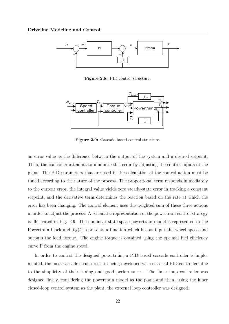
in order to adjust the process. A schematic representation of the powertrain control strategy
is illustrated in Fig. 2.9. The nonlinear state-space powertrain model is represented in the
Powertrain block and fw (t) represents a function which has as input the wheel speed and
outputs the load torque. The engine torque is obtained using the optimal fuel efficiency
curve Γ from the engine speed.
In order to control the designed powertrain, a PID based cascade controller is imple-
mented, the most cascade structures still being developed with classical PID controllers due
to the simplicity of their tuning and good performances. The inner loop controller was
designed firstly, considering the powertrain model as the plant and then, using the inner
closed-loop control system as the plant, the external loop controller was designed.
22
2.4 Driveline Control Strategies
2.4.3 Explicit MPC
Traditional control design methods such as PID or LQR cannot explicitly take into ac-count hard constraints. In contrast, a MPC algorithm solves a finite-horizon open-loopoptimization problem on-line, at each sampling instant, while explicitly taking input andstate constraints into account.
Optimal control of constrained linear and piecewise affine systems has garnered greatinterest in the research community due to the ease with which complex problems can bestated and solved. The Multi-Parametric Toolbox (MPT) provides efficient computationalmeans to obtain feedback controllers for these types of constrained optimal control problemsin a Matlab programming environment. By multi-parametric programming, a linear orquadratic optimization problem is solved off-line. The associated solution takes the formof a PWA state feedback law. In particular, the state-space is partitioned into polyhedralsets and for each of those sets the optimal control law is given as one affine function of thestate. In the online implementation of such controllers, computation of the controller actionreduces to a simple set-membership test, which is one of the reason why this method hasattracted so much interest in the research community (Kvasnica et al., 2006).
PWA systems are models for describing hybrid systems and the dynamical behavior ofsuch systems is capture by relations of the following form:
xk+1 = Aixk + Biuk + fiyk = Cixk + Diuk + gi
, (2.41)
subject to constraints on outputs, control input, and control input slew rate:
ymin ≤ yk ≤ ymaxumin ≤ uk ≤ umax
∆umin ≤ uk−uk−1 ≤∆umax
. (2.42)
The cost function used for the explicit MPC scheme is
minukk∈Z[0,N−1]
‖PNxN‖p+N−1∑k=0‖Qxxk‖p+‖Ruuk‖p
, (2.43)
where u is the vector of manipulated variables over which the optimization is performed, Nis the prediction horizon, p is the linear norm and can be 1 or ∞ for 1- and Infinity-norm,respectively. Also, Qx, Ru and PN represents the weighting matrices imposed on states,manipulated variables and terminal states, respectively.
23
Driveline Modeling and Control
2.4.4 Horizon-1 MPC based on Flexible Control Lyapunov Func-tion
Standard MPC techniques require a sufficiently long prediction horizon to guarantee stability,which makes the corresponding optimization problem too complex. Recently, a relaxationof the conventional notion of a Lyapunov function was proposed in (M.Lazar, 2009), whichresulted in a so-called flexible Lyapunov function. A first application of flexible Lyapunovfunctions in automotive control problems was presented in (Hermans et al., 2009). Thereinit was indicated that flexible Lyapunov functions can be used to design stabilizing MPCschemes with a unitary horizon, without introducing conservatism. In what follows, wedemonstrate how the theory introduced in (M.Lazar, 2009) can be employed to design ahorizon-1 MPC controller for the considered application.
2.4.4.1 Notation and Basic Definitions
Let R, R+, Z and Z+ denote the field of real numbers, the set of non-negative reals, theset of integer numbers and the set of non-negative integers, respectively. For every c ∈ Rand Π⊆ R define Π≥c := k ∈ Π | k ≥ c and similarly Π≤c, RΠ := Π and ZΠ := Z∩Π. Fora vector x ∈ Rn let ‖x‖ denote an arbitrary p-norm and let [x]i, i ∈ Z[1,n], denote the i-thcomponent of x. Let ‖x‖∞ := maxi∈Z[1,n] |[x]i|, where | · | denotes the absolute value. For amatrix Z ∈ Rm×n let ‖Z‖∞ := supx 6=0
‖Zx‖‖x‖ denote its corresponding induced matrix norm.
In ∈ Rn×n denotes the identity matrix. A function ϕ : R+ → R+ belongs to class K if itis continuous, strictly increasing and ϕ(0) = 0. A function ϕ ∈ K belongs to class K∞ iflims→∞ϕ(s) =∞.
2.4.4.2 Horizon -1 MPC
Consider the discrete-time constrained nonlinear system
xk+1 = φ(xk,uk), k ∈ Z+, (2.44)
where xk ∈ X ⊆ Rn is the state and uk ∈ U ⊆ Rm is the control input at the discrete-timeinstant k. φ : Rn×Rm→Rn is an arbitrary nonlinear, possibly discontinuous, function withφ(0,0) = 0. It is assumed that X and U are bounded sets with 0 ∈ int(X) and 0 ∈ int(U).Next, let α1,α2 ∈K∞ and let ρ ∈ R[0,1).
Definition 2.4.1 A function V : Rn→ R+ that satisfies
α1(‖x‖)≤ V (x)≤ α2(‖x‖), ∀x ∈ Rn (2.45)
24
2.4 Driveline Control Strategies
and for which there exists a, possibly set-valued, control law π : Rn⇒ U such that
V (φ(x,u))≤ ρV (x), ∀x ∈ X,∀u ∈ π(x) (2.46)
is called a control Lyapunov function (CLF) in X for system (2.44).
Consider the following inequality corresponding to (2.46):
V (xk+1)≤ ρV (xk) +λk, ∀k ∈ Z+, (2.47)
where λk is an additional decision variable which allows the radius of the sublevel set z ∈X |V (z)≤ ρV (xk)+λk to be flexible, i.e., it can increase if (2.46) is too conservative. Based oninequality (2.47) we can formulate the following optimization problem. Let α3,α4 ∈K∞ andJ : R→ R+ be a function such that α3(|λ|)≤ J(λ)≤ α4(|λ|) for all λ ∈ R and let µ ∈ R[0,1).Let Ω ⊆ X with the origin in its interior be a set where V (·) is a CLF for system (2.44).Such a region can be obtained for the desired application as the region of validity of anexplicit PWA stabilizing state feedback controller obtained for the unconstrained model.More details on how to obtain a local CLF with corresponding PWA state-feedback law formodel (2.44) are given in the next section.
Problem 2.4.2 Choose the CLF candidate V and the constants ρ ∈ R[0,1), ∆ ∈ R+ andM ∈ Z>0 off-line. At time k ∈ Z+ measure xk and minimize the cost J(λk) over uk,λksubject to the constraints
uk ∈ U, φ(xk,uk) ∈ X, λk ≥ 0, (2.48a)
V (φ(xk,uk))≤ ρV (xk) +λk, (2.48b)
λk ≤ ρ1
M (λ∗k−1 +ρk−1M ∆), ∀k ∈ Z≥1. (2.48c)
Above λ∗k denotes the optimum at time k ∈ Z+.Let π(xk) := uk ∈ Rm | ∃λk ∈ R s.t. (2.48) holds and let
φcl(x,π(x)) := φ(x,u) | u ∈ π(x).
Theorem 2.4.3 Let a CLF V in Ω be known for system (2.44). Suppose that Problem 2.4.2is feasible for all states x in X. Then the difference inclusion
xk+1 ∈ φcl(xk,π(xk)), k ∈ Z+, (2.49)
is asymptotically stable in X.
25
Driveline Modeling and Control
The proof of Theorem 2.4.3 starts from the fact that (2.48c) implies limk→∞λ∗k = 0
and then employs standard arguments for proving input-to-state stability and Lyapunovstability. For brevity a complete proof is omitted here and the interested reader is referred to(M.Lazar, 2009) for more details. However, in (M.Lazar, 2009) a more conservative conditionthan (2.48c) was used, which corresponds to setting ∆ = 0 andM = 1. As such, it is necessaryto prove that (2.48c) actually implies limk→∞λ
∗k = 0, which is accomplished in the next
lemma.
Lemma 2.4.4 Let ∆ ∈ R+ be a fixed constant to be chosen a priori and let ρ ∈ R[0,1) andM ∈ Z>0. If
0≤ λk ≤ ρ1
M (λ∗k−1 +ρk−1M ∆), ∀k ∈ Z≥1, (2.50)
then limk→∞λk = 0.
A complete proof is omitted here and, for more details, the interested reader is referred to(Caruntu, Balau et al., 2011).
2.4.5 Delta GPC
The drawback of the classic control techniques are particularly emphasized especially whenprocesses are to be run very fast and involve high sampling frequency. In this context, othercontrol strategies have been proposed to improve both the design and implementation forembedded devices.
Generalized predictive control (Camacho and Bordons, 1999), (Clarke et al., 1987) is themost popular controller among of all predictive control formulations. At high sampling rates,the conventional GPC suffers from the large number of samples that must be taken intoaccount at each sampling instant. During the last few years some research paid attentionto δ-domain GPC to emphasize the close connection between discrete time and continuoustime theory. Discrete time system analyses is usually done using q forward shift operatorand associated discrete frequency variable z. Although forward shift operator q is the mostcommonly used discrete-time operator, in some applications, the forward shift operator canlead to difficulties (Middleton and Goodwin, 1986). Unfortunately, the discrete domainsare unconnected with the continuous domain; this is because the underlying continuousdomain description cannot be obtained by setting the sample time to zero value. It hasbeen demonstrated that there is a close connection between continuous time result and δ
representation (Middleton and Goodwin, 1986). In fact, the δ domain description convergesto the continuous time counterpart for sampling period tends to zero.
26
2.4 Driveline Control Strategies
The suggestion of connecting the GPC with the advantages offered by a δ parameter-ization has been discussed in (Rostgaard et al., 1997) using an emulator in a state-spaceapproach. The δ domain emulator based GPC has been further investigated in connec-tion to discrete-time GPC in (Sera et al., 2007), using a Diophantine formulation. Thesignificant relationship in fast sampling is the ratio between the dominant time constantof the system and the sample time. For instance, many process systems where GPC is of-ten applied can be considered to be fast-sampled, due to their slowly changing dynamics(Kadirkamanathan et al., 2009).
The concept of predictive control in δ domain was first associated with GPC algorithmin continuous time domain based on a state space approach, becoming the GPC emulator(Rostgaard et al., 1997). Later, the GPC emulator has been investigated in terms of discreteGPC algorithm designed with Diophantine equations.
Considering the deterministic case of single input single output, δ domain stat- spacemodel with the known states unaffected by disturbance or noise is:
δxk=Aδxk+Bδukyk=Cδxk
, (2.51)
with xk ∈ Rn,uk ∈ Rm,yk ∈ Rp the state vector, the control vector and the output vector,respectively.
Proceed from this model, the j-th order δ derivatives state are obtained as follows(Rostgaard et al., 1997):
δjxk = Aδjxk +
j−1∑i=0
Aδj−i−1Bδδ
iuk, (2.52)
with j = 0,Ny, Ny being the prediction horizon. Using the model (2.51) the following δ
derivative predictors are estimated in the δ domain:
δjyk = CδAδjxk +
minj,Ny−1∑i=0
CδAδj−i−1Bδδ
iuk. (2.53)
In a matrix notation the expression of δ derivatives predictors can be written:
yδ= f +Guδ, (2.54)
where:
uδ = [uk δuk δ 2uk......δNu−1uk]T ,
yδ = [yk δyk δ 2yk......δNyyk]T .
(2.55)
27
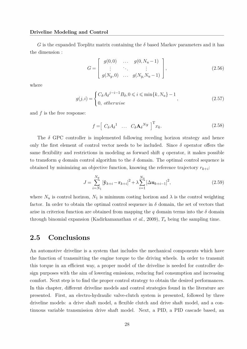
Driveline Modeling and Control
G is the expanded Toeplitz matrix containing the δ based Markov parameters and it hasthe dimension :
G=
g(0,0) . . . g(0,Nu−1)
... . . . ...g(Ny,0) . . . g(Ny,Nu−1)
, (2.56)
where
g(j, i) =
CδAδj−i−1Bδ,06 i6mink,Nu−1
0, otherwise, (2.57)
and f is the free response:
f =[CδAδ
1 . . . CδAδNy
]Txk. (2.58)
The δ GPC controller is implemented following receding horizon strategy and henceonly the first element of control vector needs to be included. Since δ operator offers thesame flexibility and restrictions in modeling as forward shift q operator, it makes possibleto transform q domain control algorithm to the δ domain. The optimal control sequence isobtained by minimizing an objective function, knowing the reference trajectory rk+i:
J =Ny∑i=N1
[yk+i− rk+i]2 +λNu∑i=1
[∆uk+i−1]2, (2.59)
where Nu is control horizon, N1 is minimum costing horizon and λ is the control weightingfactor. In order to obtain the optimal control sequence in δ domain, the set of vectors thatarise in criterion function are obtained from mapping the q domain terms into the δ domainthrough binomial expansion (Kadirkamanathan et al., 2009), Ts being the sampling time.
2.5 Conclusions
An automotive driveline is a system that includes the mechanical components which havethe function of transmitting the engine torque to the driving wheels. In order to transmitthis torque in an efficient way, a proper model of the driveline is needed for controller de-sign purposes with the aim of lowering emissions, reducing fuel consumption and increasingcomfort. Next step is to find the proper control strategy to obtain the desired performances.In this chapter, different driveline models and control strategies found in the literature arepresented. First, an electro-hydraulic valve-clutch system is presented, followed by threedriveline models: a drive shaft model, a flexible clutch and drive shaft model, and a con-tinuous variable transmission drive shaft model. Next, a PID, a PID cascade based, an
28
2.5 Conclusions
explicit MPC, a horizon-1 MPC controller based on flexible Lyapunov functions and anDelta GPC controller are presented as driveline control strategies. Starting from the modelspresented in this chapter, in what follows, more complex driveline models are developed andalso the control strategies presented in this chapter are applied in order to improve overallperformances.
29
Driveline Modeling and Control
30
Chapter 3
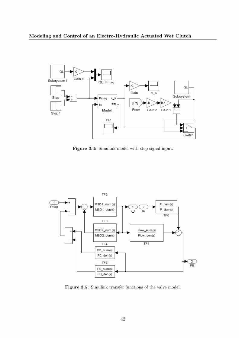
Modeling and Control of anElectro-Hydraulic Actuated WetClutch
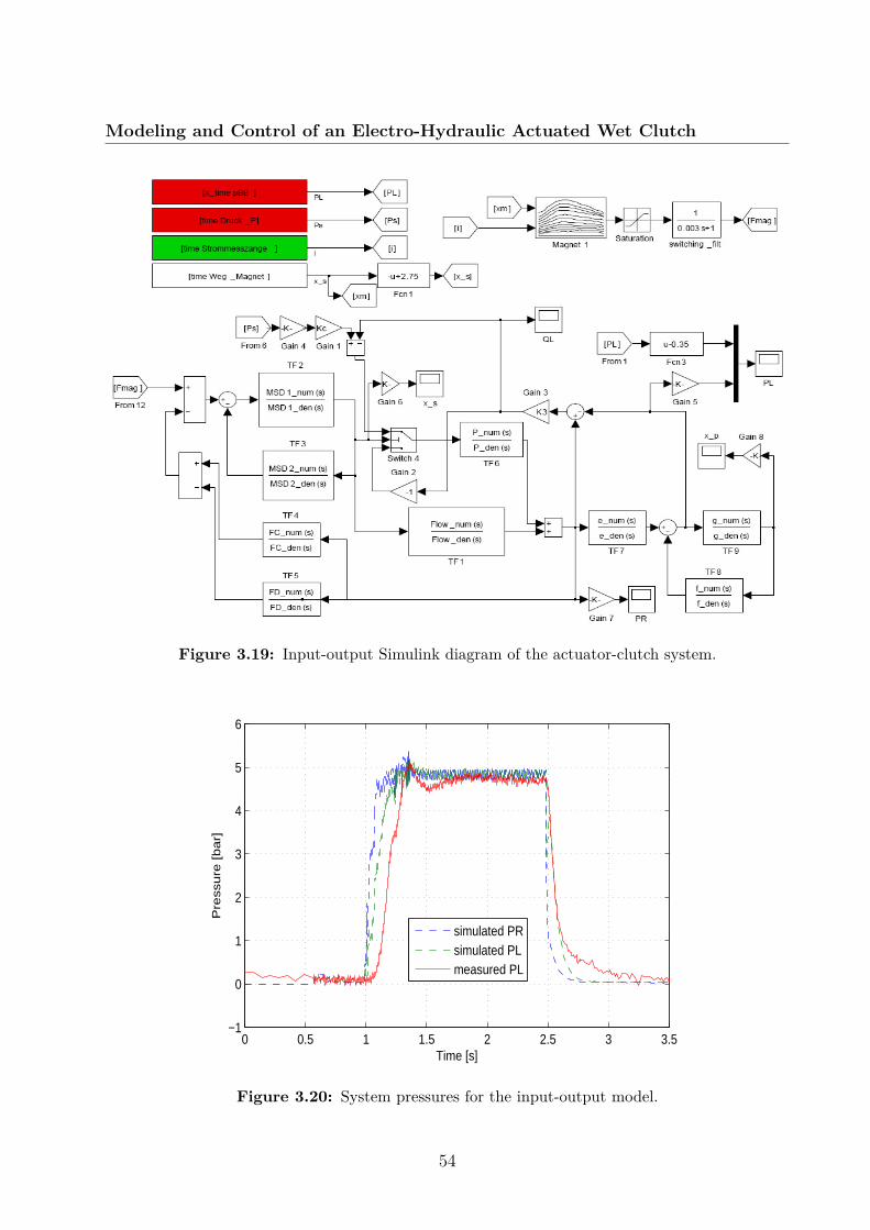
Transmission is one of the most important subsystem of an automotive powertrain, withthe basic function of transferring the engine torque to the vehicle with the desired ratiosmoothly and efficiently. The most common control devices inside the transmission areclutches and actuators, and considering that the automatic control of the clutch engagementplays a crucial role in AMT vehicles, in this chapter we deal with the problem of modelingand controlling an electro-hydraulic actuated wet clutch. First, new input-output and state-space models of an electro-hydraulic pressure reducing valve are developed and, stating fromthese, an input-output and a state space model of an electro-hydraulic actuated wet clutchare obtained. Simulators of the developed models are implemented in Matlab, and validatedwith data provided from experiments with the real valve actuator on a test bench. The testbench was provided by Continental Automotive Romania and it includes the VolkswagenDQ250 wet clutch actuated by the electro-hydraulic valve DQ500. Also, a GPC controlstrategy and for PID controllers are applied on the develop models and simulation result arebeing discussed.
3.1 Introduction
During the last few years, the interest for automated manual transmission (AMT) systemshas increased due to growing demand of driving comfort. Automated clutch actuation makesit easier for the driver, particularly in stop and go traffic, and has especially seen a recent
31
Modeling and Control of an Electro-Hydraulic Actuated Wet Clutch
growth in the European automotive industry. An AMT system consists of a manual trans-mission through the clutch disc, and an automated actuated clutch during gear shifts. Someof AMT’s largest advantages are low cost, high efficiency, reduced clutch wear and improvedfuel consumption.
Automotive actuators have become mechatronic systems in which mechanical componentscoexist with electronics and computing devices and because pressure control valves are usedas actuators in many control applications for automotive systems, a proper dynamic modelis necessary. Hydraulic control valves are devices that use mechanical motion to control asource of fluid power and are used as actuators in many control applications for automotivesystems. They vary in arrangement and complexity, depending upon their function. Themany types of valves available are best classified according to their function. Three broadfunctional types can be distinguished: directional control valves, pressure control valves andflow control valves. Pressure control valves act to regulate pressure in a circuit and may besubdivided into pressure relief valves and pressure reducing valves. Pressure relief valves,which are normally closed, open up to establish a maximum pressure and bypass excess flowto maintain the set pressure. Pressure reducing valves, which are normally open, close tomaintain a minimum pressure by restricting flow in the line. Because control valves are themechanical (or electrical) to fluid interface in hydraulic systems, their performance is underscrutiny, especially when system difficulties occurs. Therefore knowledge of the performancecharacteristics of valve is essential.
3.2 Modeling of an Electro-Hydraulic Actuated WetClutch as a Subsystem of an Automated ManualTransmission
Control valves are the mechanical (or electrical) to fluid interface in hydraulic systems,and the knowledge of their performance characteristics is essential. Pressure control valvesemploy feedback and may be properly regarded as servo control loops. Because of that, aproper dynamic design is necessary to achieve stability. Starting from equations found in(Merritt, 1967), where a single stage pressure reducing valve is modeled, in this chapter, anew concept of modeling an electro-hydraulic actuated wet clutch is presented. The workis divided into two sub-chapters, first dedicated to the modeling of a three land three waysolenoid valve actuator, and second dedicated to the modeling of the actuator-clutch system.A simulator was created for the developed models, and the results obtained were compared
32
3.2 Modeling of an Electro-Hydraulic Actuated Wet Clutch as a Subsystem ofan Automated Manual Transmission
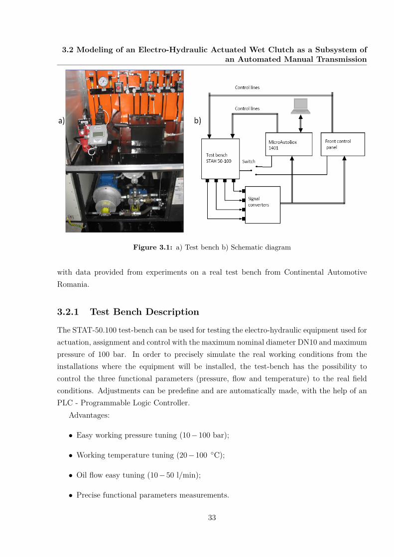
Figure 3.1: a) Test bench b) Schematic diagram
with data provided from experiments on a real test bench from Continental AutomotiveRomania.
3.2.1 Test Bench Description
The STAT-50.100 test-bench can be used for testing the electro-hydraulic equipment used foractuation, assignment and control with the maximum nominal diameter DN10 and maximumpressure of 100 bar. In order to precisely simulate the real working conditions from theinstallations where the equipment will be installed, the test-bench has the possibility tocontrol the three functional parameters (pressure, flow and temperature) to the real fieldconditions. Adjustments can be predefine and are automatically made, with the help of anPLC - Programmable Logic Controller.
Advantages:
• Easy working pressure tuning (10−100 bar);
• Working temperature tuning (20−100 C);
• Oil flow easy tuning (10−50 l/min);
• Precise functional parameters measurements.
33
Modeling and Control of an Electro-Hydraulic Actuated Wet Clutch
The STAT-50.100 test-bench is composed from the following subcomponents: hydraulictank, hydraulic oil equipment, three measurements circuits, cooling/heating oil circuit, elec-trical equipment and electronic automation equipment. Fig. 3.1.a represents the test bench,where the pressure source, the pressure reducing valve (inside of the black box) and thesensors can be easily distinguish. The schematic diagram from Fig. 3.1.b illustrated howthe test bench can be controlled either by computer, throw a software program, or directlyfrom the control panel.
3.2.2 Modeling of an Pressure Reducing Valve
Starting from the equations in (Merritt, 1967), where a single stage pressure reducing valveis modeled, in this sub-chapter, a new concept of modeling a three land three way pres-sure reducing valve used as actuator for the clutch system in the automatic transmission ofa Volkswagen vehicle is presented. Two models were developed: a linearized input-outputmodel and a state-space model then implemented in Matlab/Simulink and validated by com-paring the results with data obtained on the test-bench provided by Continental AutomotiveRomania and briefly presented in paragraph 3.2.1.
3.2.2.1 Valve Description
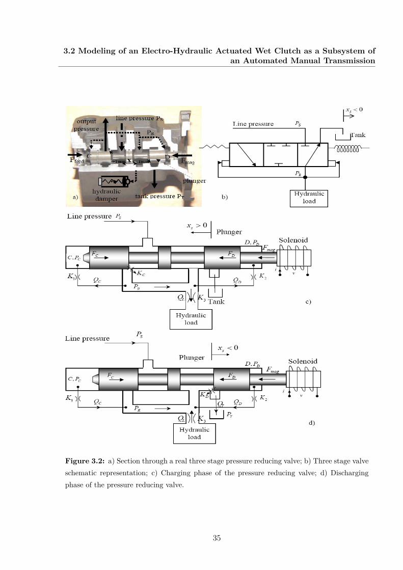
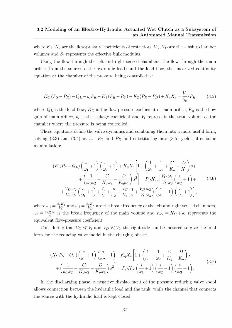
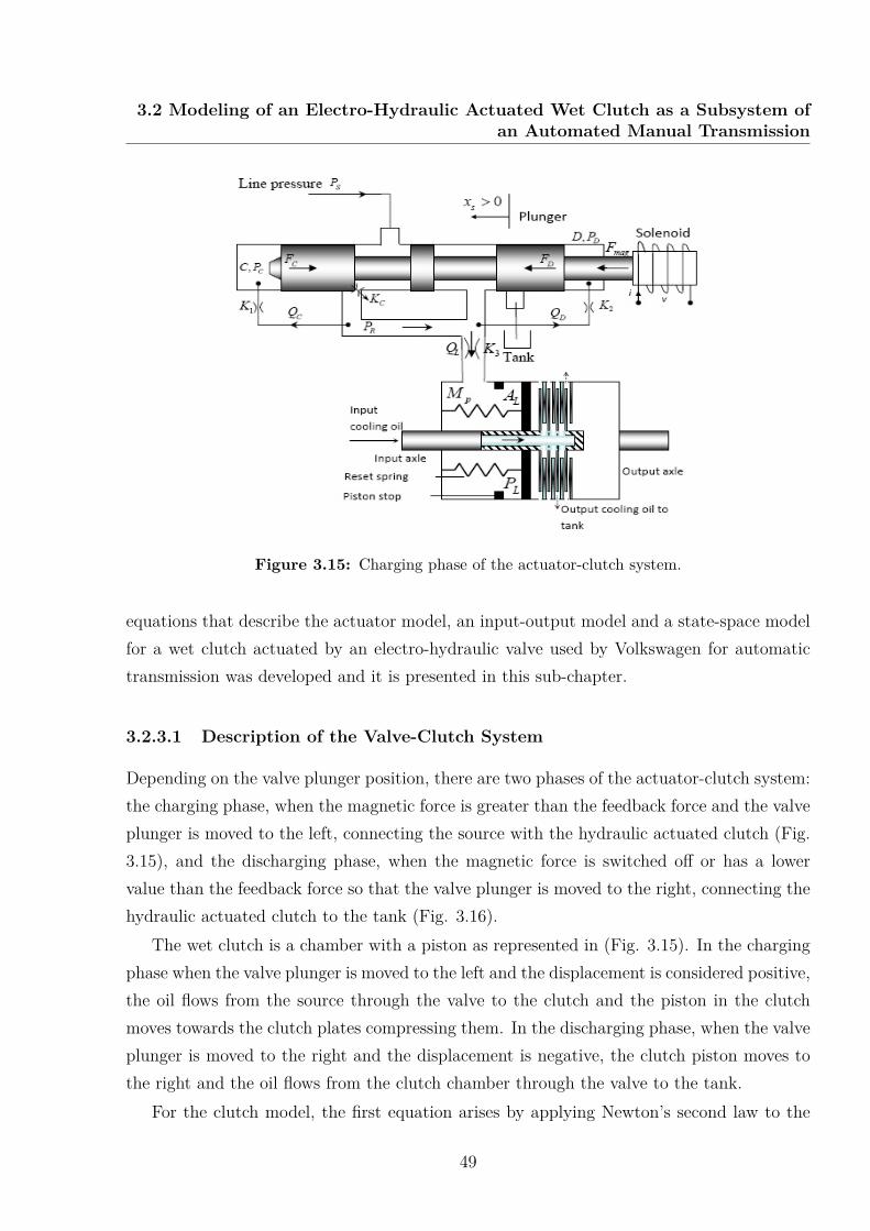
Pressure control valves employ feedback and may be properly regarded as servo control loop.Therefore proper dynamic design is necessary to achieve stability. Taking into considerationthat no model and structural description of this valve is found in literature, the electro-hydraulic valve DQ500 was mechanically sectioned in order to be analyzed. Therefore,in Fig. 3.2.a, a section through a real three stage pressure reducing valve is represented.Schematics of the three land three way pressure reducing valve are shown in Fig. 3.2.b.
A pump produces the line pressure Ps used as input for the electro-hydraulic actuatorrepresented by a pressure reducing valve. This valve releases a pressure depending on thecurrent i in the solenoid, which will have as consequence the magnetic force Fmag exertedon the valve plunger, which moves linearly within a bounded region under the effect of thisforce. Such a force is generated by a solenoid placed at one boundary of the region. Themagnetic force is a function of the solenoid current and the displacement xs, defined by:
Fmag = f(i,xs) = kai2
2(kb+xs)2 ; LSdi
dt+RSi= v, (3.1)
where ka and kb are constants, Ls is the solenoid induction, Rs the resistance and v is thesupply voltage.
34
3.2 Modeling of an Electro-Hydraulic Actuated Wet Clutch as a Subsystem ofan Automated Manual Transmission
Figure 3.2: a) Section through a real three stage pressure reducing valve; b) Three stage valveschematic representation; c) Charging phase of the pressure reducing valve; d) Dischargingphase of the pressure reducing valve.
35
Modeling and Control of an Electro-Hydraulic Actuated Wet Clutch
The pressure to be controlled PR is sensed on the spool end areas C and D and comparedwith the magnetic force which actuates on the plunger. The feedback force Ffeed = FC−FDis the difference between the force applied on the left sensed pressure chamber FC , and theforce applied on the right sensed pressure chamber FD.
The difference in force is used to actuate the spool valve which controls the flow tomaintain the pressure at the set value. In the charging phase, illustrated in Fig. 3.2.c, themagnetic force is greater than the feedback force and moves the plunger to the left (xs > 0),connecting the source with the hydraulic load. In the discharging phase, illustrated in Fig.3.2.d, the feedback force becomes grater than the magnetic force and the plunger is movedto the right (xs < 0); the connection between the source and the hydraulic load is closed,the hydraulic load being connected to the tank.
Using the magnetic force and the feedback force it results a force balance which describesthe spool motion and the output pressure. This equation of force balance is the same forboth positive and negative displacement of the spool:
Fmag−CPC +DPD =Mvs2Xs+KeXs, (3.2)
where PC represents the pressure in the left sensed chamber that acts on the (C) area, PDrepresents the pressure in the right sensed chamber that acts on the (D) area, Mv is thespool mass, Ke = 0.43w(PS0˘PR0) represents the flow force spring rate calculated for thenominal pressures PS0,PR0, w represents the area gradient of the main orifice, Xs = Xs(s)is the Laplace transform of the spool displacement and s represents the Laplace operator.In Fig. 3.2.a, a hydraulic damper that acts to reduce the input pressure spike, which hasnegative effects on the output pressure, is also represented.
3.2.2.2 Input-Output Model
The charging phase of the pressure reducing valve has been illustrated in Fig. 3.2.c. Apositive displacement of the spool allows connection between the source and the hydraulicload, while the channel that connects the hydraulic load with the tank is kept closed.
The linearized continuity equation from (Merritt, 1967) was used to describe the dynam-ics from the sensed pressure chambers:
QC =K1 (PR−PC) = VCβesPC −CsXs, (3.3)
QD =K2 (PR−PD) = VDβesPD +DsXs, (3.4)
36
3.2 Modeling of an Electro-Hydraulic Actuated Wet Clutch as a Subsystem ofan Automated Manual Transmission
whereK1, K2 are the flow-pressure coefficients of restrictors, VC , VD are the sensing chambervolumes and βe represents the effective bulk modulus.
Using the flow through the left and right sensed chambers, the flow through the mainorifice (from the source to the hydraulic load) and the load flow, the linearized continuityequation at the chamber of the pressure being controlled is:
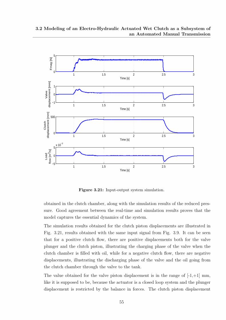
where QL is the load flow, KC is the flow-pressure coefficient of main orifice, Kq is the flowgain of main orifice, kl is the leakage coefficient and Vt represents the total volume of thechamber where the pressure is being controlled.
These equations define the valve dynamics and combining them into a more useful form,solving (3.3) and (3.4) w.r.t. PC and PD and substituting into (3.5) yields after somemanipulation:
(KCPS−QL)(s
ω1+ 1
)(s
ω2+ 1
)+KqXs
[1 +
(1ω1
+ 1ω2
+ C
Kq− D
Kq
)s+
+(
1ω1ω2
+ C
Kqω2− D
Kqω1
)s2]
= PRKce
[VCVt
ω1ω3
(s
ω2+ 1
)+
+VDVt
ω2ω3
(s
ω1+ 1
)+(
1 + s
ω3+ VCVt
ω1ω3
+ VDVt
ω2ω3
)(s
ω1+ 1
) (s
ω2+ 1
)],
(3.6)
where ω1 = βeK1VC
and ω2 = βeK2VD
are the break frequency of the left and right sensed chambers,ω3 = βeKce
Vtis the break frequency of the main volume and Kce = KC + kl represents the
equivalent flow-pressure coefficient.Considering that VC Vt and VD Vt, the right side can be factored to give the final
form for the reducing valve model in the charging phase:
(KCPS−QL)(s
ω1+ 1
)(s
ω2+ 1
)+KqXs
[1 +
(1ω1
+ 1ω2
+ C
Kq− D
Kq
)s+
+(
1ω1ω2
+ C
Kqω2− D
Kqω1
)s2]
= PRKce
(s
ω1+ 1
)(s
ω2+ 1
)(s
ω3+ 1
).
(3.7)
In the discharging phase, a negative displacement of the pressure reducing valve spoolallows connection between the hydraulic load and the tank, while the channel that connectsthe source with the hydraulic load is kept closed.
37
Modeling and Control of an Electro-Hydraulic Actuated Wet Clutch
The linearized continuity equations at the sensed pressure chambers for the dischargingphase of the valve, illustrated in Fig. 3.2.d, are:
−QC =K1 (PC −PR) =−VCβesPC +CsXs, (3.8)
−QD =K2 (PD−PR) =−VDβesPD−DsXs. (3.9)
Using the flow through the left and right sensed chambers, the flow through the mainorifice (from the hydraulic load to the tank) and the load flow, the linearized continuityequation obtained for the chamber of the pressure being controlled is:
where KD is the flow-pressure coefficient of main orifice and PT represents the tank pressure.Combining these equations into a more useful form, solving (3.8) and (3.9) for PC and
PD and substituting into (3.10) yields after some manipulation:
(KDPT +QL)(s
ω1+ 1
)(s
ω2+ 1
)+KqXs
[1 +
(1ω1
+ 1ω2
+ C
Kq− D
Kq
)s+
+(
1ω1ω2
+ C
Kqω2− D
Kqω1
)s2]
= PRKce
[VCVt
ω1ω3
(s
ω2+ 1
)+
+VDVt
ω2ω3
(s
ω1+ 1
)+(
1 + s
ω3+ VCVt
ω1ω3
+ VDVt
ω2ω3
)(s
ω1+ 1
)(s
ω2+ 1
)],
(3.11)
In an entire analogue manner, again making the assumption that VC Vt and VD Vt
like for the charging phase model and considering KD =KC the final form for the reducingvalve in the discharging phase was obtained:
(KDPT +QL)(s
ω1+ 1
)(s
ω2+ 1
)+KqXs
[1 +
(1ω1
+ 1ω2
+ C
Kq− D
Kq
)s+
+(
1ω1ω2
+ C
Kqω2− D
Kqω1
)s2]
= PRKce
(s
ω1+ 1
)(s
ω2+ 1
)(s
ω3+ 1
).
(3.12)
Equations (3.1), (3.2), (3.3), (3.4), (3.5) and (3.7) for the charging phase of the valve,and equations (3.1), (3.2), (3.8), (3.9), (3.10) and (3.12) for the discharging phase of the
38
3.2 Modeling of an Electro-Hydraulic Actuated Wet Clutch as a Subsystem ofan Automated Manual Transmission
Figure 3.3: Transfer function block diagram of the pressure reducing valve.
valve, define the pressure reducing valve dynamics and can be used to construct the transferfunction block diagram represented in Fig. 3.3. Also, the following notation was made:
G(s) =Kq
Kce
[1 +
(1ω1
+ 1ω2
+ CKq− D
Kq
)s+
(1
ω1ω2+ CKqω2
− DKqω1
)s2]
(1 + s
ω1
)(1 + s
ω2
)(1 + s
ω3
) . (3.13)
Considering the resulting force between the magnetic and the feedback force:
F1 = Fmag−CPC +DPD, (3.14)
solving PC and PD from the linearized continuity equations (3.3), (3.4) and substituting inthe force balance equation (3.2), the following equation was obtained:
Fmag−CK1PR+CsXs(
sω1
+ 1)K1
+DK2PR−DsXs(
sω2
+ 1)K2
=Mvs2Xs+KeXs. (3.15)
After some manipulations, where it was considered that ωm =√KeMv
, representing the
39
Modeling and Control of an Electro-Hydraulic Actuated Wet Clutch
mechanical natural frequency, and substituting (3.14) into (3.2) yields:
F1−
C2
K1s(
sω1
+ 1) +
D2
K2s(
sω2
+ 1)Xs =Ke
(s2
ω2m
+ 1)Xs, (3.16)
where
F1 = Fmag−
Csω1
+ 1 + Dsω2
+ 1
PR, (3.17)
illustrating the closed loop model from Fig. 3.3 for the displacement xs. A switch is used inorder to commutate between the two phases of the pressure reducing valve. Like seen in Fig.3.3, switching between the charging and the discharging phase can be realized by selectingdifferent disturbances for positive and negative displacement of the spool.
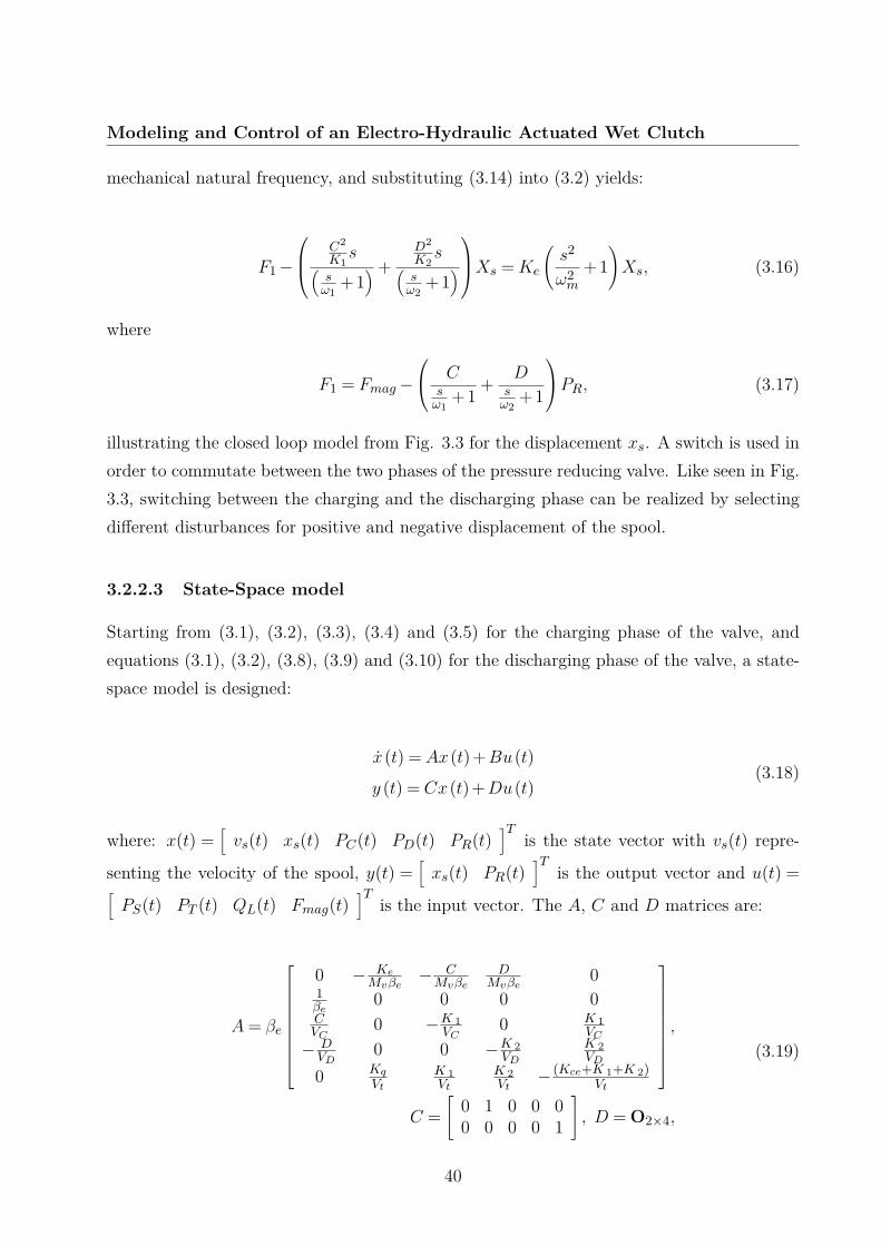
3.2.2.3 State-Space model
Starting from (3.1), (3.2), (3.3), (3.4) and (3.5) for the charging phase of the valve, andequations (3.1), (3.2), (3.8), (3.9) and (3.10) for the discharging phase of the valve, a state-space model is designed:
x(t) = Ax(t) +Bu(t)
y (t) = Cx(t) +Du(t)(3.18)
where: x(t) =[vs(t) xs(t) PC(t) PD(t) PR(t)
]Tis the state vector with vs(t) repre-
senting the velocity of the spool, y(t) =[xs(t) PR(t)
]Tis the output vector and u(t) =[
PS(t) PT (t) QL(t) Fmag(t)]T
is the input vector. The A, C and D matrices are:
A= βe
0 − KeMvβe
− CMvβe
DMvβe
01βe
0 0 0 0CVC
0 −K 1VC
0 K 1VC
− DVD
0 0 −K 2VD
K 2VD
0 Kq
Vt
K 1Vt
K 2Vt
− (Kce+K 1+K 2)Vt
,
C =[
0 1 0 0 00 0 0 0 1
], D = O2×4,
(3.19)
40
3.2 Modeling of an Electro-Hydraulic Actuated Wet Clutch as a Subsystem ofan Automated Manual Transmission
and the matrix B has the B1 expression in the charging phase (for xs > 0) and the B2
expression in the discharging phase (for xs < 0), where:
B1 = βe
0 0 0 1
Mvβe
0 0 0 00 0 0 00 0 0 0KCVt
0 − 1Vt
0
, B2 = βe
0 0 0 1
Mvβe
0 0 0 00 0 0 00 0 0 00 KC
Vt
1Vt
0
. (3.20)
This model is more precise because no approximations were used, as for the input-outputmodel.
3.2.2.4 Simulators for the Pressure Reducing Valve
In this section two simulators that were designed starting from the models previously de-scribed are developed in Matlab/Simulink program. Parameter values used for testing inSimulink are presented in Table A.1. Dimensional parameters were measured directly onthe sectioned valve and the flow coefficients were determined through experiments with thereal valve on a test bench at Continental Automotive Romania. The models were validatedby comparing the results with data obtained on a real test-bench provided by ContinentalAutomotive Romania.
For testing purposes a Simulink model illustrated in Fig. 3.4 was created, using as in-put a step signal. The commutation between the charging and the discharging phase wassimulated by a switch that connects different perturbation depending on the value of thedisplacement. In Fig. 3.4 two subsystems were used: one noted Model and representing thetransfer functions of the reducing valve model (Fig. 3.5) that were represented as a blockdiagram in Fig. 3.3, and one noted as Load Flow representing the load flow.
For a step signal as the magnetic force and a sequence of pulses as the load flow rep-resented in Fig. 3.6, the results obtained for spool displacement and reduced pressure arepresented in Fig. 3.7. For modeling the load flow needed to actuate the clutch, two im-pulse signals, a positive one and a negative one, for 20 ms with a value of 10−4m3/s wereconsidered, value determined from measurements on the test bench.
The displacement follows the step input behavior while the reducing pressure has almostthe same value like the reference signal. The model shows good performance, being stablefor input signals variations.
1. Input-output model simulation
41
Modeling and Control of an Electro-Hydraulic Actuated Wet Clutch
Figure 3.4: Simulink model with step signal input.
Figure 3.5: Simulink transfer functions of the valve model.
42
3.2 Modeling of an Electro-Hydraulic Actuated Wet Clutch as a Subsystem ofan Automated Manual Transmission
0 0.5 1 1.5 2 2.5 3 3.5 4 4.5−1
0
1
2
3
4
5
Time [s]
Fm
g[N
], Q
L [1
04 *m3 /s
]
QLFmag
Figure 3.6: Magnetic force and load flow.
0 0.5 1 1.5 2 2.5 3 3.5 4 4.5−1
0
1
2
3
4
5
6
7
Time [s]
Dis
plac
emen
t [m
], P
ress
ure
[bar
]
DisplacementPressure
Figure 3.7: Spool displacement and reduced pressure.
43
Modeling and Control of an Electro-Hydraulic Actuated Wet Clutch
Figure 3.8: Input-output Simulink model.
In order to validate the results obtained for the solenoid valve actuator, a Simulinkmodel (represented in Fig. 3.8) was created, using a magnetic force as input (Magnetblock). The magnetic force block implements the connection between electric currenttrough solenoid and magnetic force generated by the magnetic flux. A force sensor wasutilized to measure the magnetic force and the results were used in a form of a twodimensional look-up table, designed at Continental Automotive Romania for this typeof valve.
The blocks in the upper part of the model (time_Druck_A, time_Druck_P , ti-me_Strommesszange and time_Weg_Magnet) represent the real data (correspond-ing to PR, Ps, i and xs respectively) obtained from experiments made on the test benchat Continental Automotive Romania with this type of valve. The gains in the model
44
3.2 Modeling of an Electro-Hydraulic Actuated Wet Clutch as a Subsystem ofan Automated Manual Transmission
0 0.2 0.4 0.6 0.8 1 1.2 1.4 1.6−1
0
1
2
3
4
5
6
7
8
Time [s]
Fm
ag [N
], cu
rent
[A]
Fmagi − curent
Figure 3.9: Current and magnetic force used as input signals.
are used to transform the values of the parameters that are in international units inother units used for display (meter to millimeter for the spool displacement and Pascalto bar for the reduced pressure).
In Fig. 3.8 the saturation block was used to allow only positive values for the magneticforce and the filter (switching_filt) to eliminate the high frequencies caused by thelook-up table. In Fig. 3.9 a real input signal is illustrated, represented either by themagnetic force or by the current used to obtain the magnetic force through the look-uptable.
The results of the simulations are presented in Figs. 3.10 and 3.11, where the spooldisplacement and the reduced pressure were compared with real data obtained fromexperiments made on a test bench with the input signal from Fig. 3.9. It can beseen that the simulated displacement of the spool has even smaller variations than themeasured displacement while the behavior is the same.
Concerning the reduced pressure, the experimental results reveal that the simulatedpressure follows the measured pressure behavior, having in the steady state an irre-levant offset. The amplitude of the simulated pressures variations in steady state islower than the amplitude of the measured pressures variations.
2. State-space model simulator
45
Modeling and Control of an Electro-Hydraulic Actuated Wet Clutch
0 0.2 0.4 0.6 0.8 1 1.2 1.4 1.6−0.4
−0.2
0
0.2
0.4
0.6
0.8
1
Time [s]
Dis
plac
emen
t [m
m]
measuredsimulated
Figure 3.10: Compared spool displacements for input-output model .
0 0.2 0.4 0.6 0.8 1 1.2 1.4 1.6−2
0
2
4
6
8
10
12
14
Time [s]
Pre
ssur
e [b
ar]
measuredsimulated
Figure 3.11: Compared reducing pressures for input-output model.
46
3.2 Modeling of an Electro-Hydraulic Actuated Wet Clutch as a Subsystem ofan Automated Manual Transmission
Figure 3.12: State-space Simulink model.
The state-space model was represented in Simulink as shown in Fig. 3.12, where asimilar switch as in the input-output model was used in order to commutate the reducedpressure between the charging and the discharging phases. The results obtained forthe spool displacement using the state-space model, are similar to those obtained usingthe input-output model and are represented in Fig. 3.13.
Fig. 3.14 illustrates the difference between the simulated and the measured reducedpressures. It can be seen that the amplitude of the simulated pressures variations insteady state is lower than the amplitude of the measured pressures variations. Also,the simulated pressure has in steady state a slight offset.
3.2.3 Modeling of the Electro-Hydraulic Actuated Wet ClutchSystem
In previous sub-chapter, two models for an electro-hydraulic actuator were developed: aninput-output model, where simplifications were made in order to obtain a suitable transferfunction to be implemented in Matlab-Simulink, and a state-space model. Starting from the
47
Modeling and Control of an Electro-Hydraulic Actuated Wet Clutch
0 0.2 0.4 0.6 0.8 1 1.2 1.4 1.6−0.4
−0.2
0
0.2
0.4
0.6
0.8
1
Time [s]
Dis
plac
emen
t [m
m]
measuredsimulated
Figure 3.13: Compared spool displacements for state-space model.
0 0.2 0.4 0.6 0.8 1 1.2 1.4 1.6−2
0
2
4
6
8
10
12
14
Time [s]
Pre
ssur
e [b
ar]
measuredsimulated
Figure 3.14: Compared reducing pressures for state-space model.
48
3.2 Modeling of an Electro-Hydraulic Actuated Wet Clutch as a Subsystem ofan Automated Manual Transmission
Figure 3.15: Charging phase of the actuator-clutch system.
equations that describe the actuator model, an input-output model and a state-space modelfor a wet clutch actuated by an electro-hydraulic valve used by Volkswagen for automatictransmission was developed and it is presented in this sub-chapter.
3.2.3.1 Description of the Valve-Clutch System
Depending on the valve plunger position, there are two phases of the actuator-clutch system:the charging phase, when the magnetic force is greater than the feedback force and the valveplunger is moved to the left, connecting the source with the hydraulic actuated clutch (Fig.3.15), and the discharging phase, when the magnetic force is switched off or has a lowervalue than the feedback force so that the valve plunger is moved to the right, connecting thehydraulic actuated clutch to the tank (Fig. 3.16).
The wet clutch is a chamber with a piston as represented in (Fig. 3.15). In the chargingphase when the valve plunger is moved to the left and the displacement is considered positive,the oil flows from the source through the valve to the clutch and the piston in the clutchmoves towards the clutch plates compressing them. In the discharging phase, when the valveplunger is moved to the right and the displacement is negative, the clutch piston moves tothe right and the oil flows from the clutch chamber through the valve to the tank.
For the clutch model, the first equation arises by applying Newton’s second law to the
49
Modeling and Control of an Electro-Hydraulic Actuated Wet Clutch
Figure 3.16: Discharging phase of the actuator-clutch system.
forces on the piston, resulting:
ALPL =Mps2xp+Kxp, (3.21)
where AL is the area of piston, PL the pressure from the piston chamber, xp the pistondisplacement, Mp the total mass of the piston and K is the load spring gradient of thepiston.
3.2.3.2 Input-Output Model
Applying the continuity equation to the piston chamber yields:
QL =K3 (PR−PL) = VLβesPL+ALsxp, (3.22)
for the charging phase of the system, and:
−QL =K3 (PL−PR) =−VLβesPL−ALsxp, (3.23)
for the discharging phase of the system, where K3 is the flow-pressure coefficient of the pipefrom valve actuator to the clutch and VL is the piston chamber volume.
50
3.2 Modeling of an Electro-Hydraulic Actuated Wet Clutch as a Subsystem ofan Automated Manual Transmission
Figure 3.17: Transfer function block diagram of the actuator-clutch system.
Equations (3.22) and (3.23), for the charging phase of the clutch, and (3.22) and (3.24)for the discharging phase of the clutch, together with the equations that describe the valveplunger dynamics, define the electro-hydraulic actuated wet clutch system dynamic model.
Starting from these equations, a schematic diagram of the transfer functions for theactuator-clutch system was created and represented in Fig. 3.17. It can be seen that a switchblock was used in order to commutate between the two phases that describe the functionalityof the actuator, the charging and the discharging phase. The sign of the displacement of theplunger was used as the switch parameter, thus selecting different perturbations for positiveor negative displacements of the plunger.
3.2.3.3 State-Space Model
Combining the equations (3.1), (3.2), (3.3), (3.4), (3.5), (3.21) and (3.22) that describe thedynamics of the system in the charging phase, and equations (3.1), (3.2), (3.8), (3.9), (3.10), (3.21) and (3.23) that describe the dynamics of the system in the discharging phase, thestate-space model of the electro-hydraulic actuated clutch is design according to:
x(t) = Ax(t) +Bu(t)
y (t) = Cx(t) +Du(t)(3.24)
51
Modeling and Control of an Electro-Hydraulic Actuated Wet Clutch
The state vector is represented by x(t), u(t) is the input vector, and y (t) is consideredto be the output of the system:
u(t) =[PS (t) PT (t) Fmag (t)
]T,
x(t) =[vs (t) xs (t) vp (t) xp (t) PC (t) PD (t) PR (t) PL (t)
]T,
y(t) =[xs (t) xp (t) PR (t) PL (t).
]T (3.25)
Instead of the solenoid current, the magnetic force was used as input because it is anonlinear function of the current, the relation between the magnetic force and the currenttogether with the plunger displacement being implemented in a form of a two dimensionallook-up table designed at Continental Automotive Romania, for this type of valve. Thematrix A is the same for both charging and discharging phase of the actuator-clutch systemand we consider Ksum =Kce+K1 +K2 +K3 in:
A=
0 −KeMv
0 0 − CMv
DMv
0 01 0 0 0 0 0 0 00 0 0 K
Mt0 0 0 AL
Mt
0 0 1 0 0 0 0 0CβeVc
0 0 0 −K1βeVc
0 K1βeVc
0−Dβe
VD0 0 0 0 −K2βe
VD
K2βeVD
00 Kqβe
Vt0 0 K1βe
Vt
K2βeVt
−KsumβeVt
K3βeVt
0 0 ALβeVL
0 0 0 K3βeVL
−K3βeVL
, (3.26)
while different values of the B matrix are used: B1 for the charging phase of the system andB2 for the discharging phase of the electro-hydraulic actuated clutch:
B1 =
0 0 1Mv
0 0 00 0 00 0 00 0 00 0 0
KcβeVt
0 00 0 0
,B2 =
0 0 1Mv
0 0 00 0 00 0 00 0 00 0 00 Kcβe
Vt0
0 0 0
. (3.27)
Starting from the equations that illustrates the mathematical model, a block diagramfor the actuator-clutch system was created and represented in Fig. 3.18. It can be seenthat a switch block was used, relative to the sign of the plunger displacement, in order tocommutate between the two phases that describe the functionality of the actuator: B1 forthe charging phase of the system and B2 for the discharging phase.
52
3.2 Modeling of an Electro-Hydraulic Actuated Wet Clutch as a Subsystem ofan Automated Manual Transmission
Figure 3.18: State-space block diagram of the actuator-clutch system.
3.2.3.4 Simulators for the Electro-Hydraulic Actuated Wet Clutch
In order to validate the model obtained for the electro-hydraulic actuated clutch, a simula-tor was designed and developed in Matlab/Simulink starting from the mathematical modeldescribed previously. The parameters used in the model of the valve actuated wet clutch,summarized in Table A.1, are estimated experimentally at Continental Automotive Romaniausing a test-bench, or are already given by the manufacturer. A test-bench which includesthe Volkswagen DQ250 wet clutch actuated by the electro-hydraulic valve DQ500 was pro-vided by Continental Automotive Romania. Experiments made on the test-bench allowedobtaining the parameters used in simulations for the electro-hydraulic actuator: the volumesof the actuator chambers, the left and right areas of the valve plunger, the flow-pressurecoefficients. The test-bench also provides measurements for the outputs of the system, rep-resented by the valve plunger displacement and the clutch pressure which are used in orderto validate the implemented simulator.
1. Input-output model simulation
The input-output model of the actuator-clutch system was implemented in Matlab/Si-mulink like presented in Fig. 3.19 and it can be seen that the switch commutatesbetween the two phases of the system by connecting different perturbations.
Following experiments made on the test-bench from Continental Automotive Romania,using as input the solenoid current i, respectively the magnetic force Fmag obtainedthrough the look-up table, and represented in Fig. 3.9, the real-time clutch pressureresponse from Fig. 3.20 was obtained. The input-output model simulation results arevalidated due to similar behavior obtained for the pressure in the clutch chamber. Fig.3.20 shows the comparison between measurements and simulations for the pressure
53
Modeling and Control of an Electro-Hydraulic Actuated Wet Clutch
Figure 3.19: Input-output Simulink diagram of the actuator-clutch system.
0 0.5 1 1.5 2 2.5 3 3.5−1
0
1
2
3
4
5
6
Time [s]
Pre
ssu
re [
ba
r]
simulated PRsimulated PLmeasured PL
Figure 3.20: System pressures for the input-output model.
54
3.2 Modeling of an Electro-Hydraulic Actuated Wet Clutch as a Subsystem ofan Automated Manual Transmission
1 1.5 2 2.5 30
5
Time [s]
Fm
ag
[N
]
1 1.5 2 2.5 3−1
0
1
Time [s]
Va
lve
d
isp
lace
me
nt [m
m]
1 1.5 2 2.5 30
500
Time [s]
Clu
tch
d
isp
lace
me
nt [m
m]
1 1.5 2 2.5 3−5
0
5x 10
−3
Time [s]
Lo
ad
flo
w [m
3/s
]
Figure 3.21: Input-output system simulation.
obtained in the clutch chamber, along with the simulation results of the reduced pres-sure. Good agreement between the real-time and simulation results proves that themodel captures the essential dynamics of the system.
The simulation results obtained for the clutch piston displacements are illustrated inFig. 3.21, results obtained with the same input signal from Fig. 3.9. It can be seenthat for a positive clutch flow, there are positive displacements both for the valveplunger and the clutch piston, illustrating the charging phase of the valve when theclutch chamber is filled with oil, while for a negative clutch flow, there are negativedisplacements, illustrating the discharging phase of the valve and the oil going fromthe clutch chamber through the valve to the tank.
The value obtained for the valve piston displacement is in the range of [-1,+1] mm,like it is supposed to be, because the actuator is a closed loop system and the plungerdisplacement is restricted by the balance in forces. The clutch piston displacement
55
Modeling and Control of an Electro-Hydraulic Actuated Wet Clutch
Figure 3.22: State-space Simulink diagram of the actuator-clutch system.
goes to 400 mm. and it can be seen that it is directly influenced by the value of theload flow.
2. State-Space Model Simulation
The state-space model of the actuator-clutch system was implemented in Matlab/Simulinklike presented in Fig. 3.22 and it can be seen that the switch commutates between thetwo phases of the system by connecting different perturbations.
Like in the case of the input-output model, the state-space model is validated due tosimilar behavior obtained for the pressure in the clutch chamber. Fig. 3.23 shows thecomparison between measurements and simulations for the pressure obtained in theclutch chamber, along with the simulation results of the reduced pressure.
The behavior obtained for the valve plunger displacement and the clutch piston dis-placement represented in Fig. 3.24, are similar with the behavior obtained for theinput-output model. In the state-space model developed in this paper for the actuator-
56
3.3 Control of the Electro-Hydraulic Actuated WetClutch as a Subsystem of an Automated Manual Transmission
0 0.5 1 1.5 2 2.5 3 3.5−1
0
1
2
3
4
5
6
Time [s]
Pre
ssu
re [
ba
r]
simulated PRsimulated PLmeasured PL
Figure 3.23: System pressures for the state-space model.
clutch system, the clutch flow, which is also illustrated in Fig. 3.24, was obtained as adifference between the pressure from the valve and the clutch pressure.
The value obtained for the valve piston displacement is again in the range of [-1,+1]mm, because the actuator is a closed loop system and the plunger displacement isrestricted by the balance in forces. On the other hand, the clutch is an open loopsystem, with no feedback, resulting a high value of the piston displacement which canbe further limited by designing a proper controller for the electro-hydraulic actuatedwet clutch.
3.3 Control of the Electro-Hydraulic Actuated WetClutch as a Subsystem of an Automated ManualTransmission
Starting from the electro-hydraulic actuated wet clutch system input-output model presentedin the previous section, an analytical designed PID controller, with the help of the poleplacement method and a GPC controller are presented and the results are compared anddiscussed.
57
Modeling and Control of an Electro-Hydraulic Actuated Wet Clutch
1 1.5 2 2.5 30
5
Time [s]
Fm
ag
[N
]
1 1.5 2 2.5 3−1
0
1
Time [s]
Va
lve
d
isp
lace
me
nt [m
m]
1 1.5 2 2.5 30
500
Time [s]
Clu
tch
dis
pla
ce
me
nt [m
]
1 1.5 2 2.5 3−5
0
5x 10
−3
Time [s]
Lo
ad
flo
w [m
3/s
]
Figure 3.24: State-space system simulation.
3.3.1 Generalized Predictive Control
Predictive control techniques are of a particular interest from the point of view of bothbroad applicability and implementation simplicity, being applied on large scale in industryprocesses, having good performances and being robust at the same time.
Consider the plant described by the CARIMA (Controlled AutoRegressive IntegratedMoving Average) model (Camacho and Bordons, 2004):
A(z−1
)y (k) =B
(z−1
)u(k−1) +
e(k)C(z−1
)D (z−1) , (3.28)
where e(k) is white noise with zero mean value, u is the input voltage, y(k) is the clutchdisplacement, A
(z−1
)and B
(z−1
)are the system polynomials with the degrees nA and nB,
and C(z−1
)= 1 and D
(z−1
)= 1− z−1 are the disturbances polynomials.
58
3.3 Control of the Electro-Hydraulic Actuated WetClutch as a Subsystem of an Automated Manual Transmission
The input output model of the electro-hydraulic actuated wet clutch was implementedin Matlab/Simulink, and, in order to apply a control strategy, the input of the system wasconsidered to be the v voltage, while the output of the system is the clutch piston displace-ment. The actuator-clutch system was identified with an ARX equivalent one employing thesimulation model, utilizing as input a PRBS (PseudoRandom Binary Sequence) signal:
A(z−1
)= 1−1.781z−1 + 0.8039z−2,
B(z−1
)= 0.00003312z−1 + 0.0001122z−2,
(3.29)
and the disturbances polynomials were considered to be C(z−1
)= 1 and D
(z−1
)= 1−z−1
for obtaining a zero steady-state error.The prediction model is given by
y (k+ j|k) =Gj(z−1
)D(z−1
)z−1u(k+ j)+
+Hj
(z−1
)D(z−1
)C (z−1) u(k−1) +
Fj(z−1
)C (z−1) y (k)
, (3.30)
with j = hi,hp, where hi is the minimum prediction horizon and hp is the prediction horizon.u(k+ j− 1 |k ), j = 1,hc is the future control, computed at time k and y (k+ j|k) are thepredicted values of the output, hc being the control horizon.
The two Diophantine equations presented in (Camacho and Bordons, 2004) are used todetermine the polynomials Fj
(z−1
), Gj
(z−1
)and Hj
(z−1
).
Considering as inputs D(z−1)u(k) and collecting the j-step predictors in a matrix nota-tion, the prediction model can be written as
y =Gud+ y0, (3.31)
where y represents the free response and matrix G is given in (Camacho and Bordons, 2004).The objective function is based on the minimization of the tracking error and on the
minimization of the controller output, the control weighting factor λ being introduced inorder to make a trade-off between these objectives
J = (Gud+ y0−w)T (Gud+ y0−w) +λudTud, (3.32)
subject to D(z−1)u(k+ i) = 0 for i ∈ [hc,hp−1], where w is the reference trajectory vectorwith the components w(k+j |k ), j = hi,hp. Minimizing the objective function (∂J/∂ud = 0),the optimal control sequence yields as
u∗d =(GTG+λIhc
)−1GT [w− y0] . (3.33)
59
Modeling and Control of an Electro-Hydraulic Actuated Wet Clutch
0 0.1 0.2 0.3 0.4 0.5 0.6 0.7 0.8 0.9 10
0.5
1
1.5
2
2.5
3
3.5
4x 10
−3
Time [s]
Disp
lacem
ent [
mm
]
referencedisplacement
Figure 3.25: GPC results.
Using the receding horizon principle and considering that γj , j = hi,hp are the elementsof the first row of the matrix
(GTG+λIhc
)−1GT, the following control algorithm results:
D(z−1
)u(k) =
hp∑j=hi
γj [w (k+ j |k )− y0 (k+ j |k )]. (3.34)
The determined controller of the electro-hydraulic actuated wet clutch system was imple-mented in Matlab/Simulink. A reference signal was applied for the clutch piston displace-ment and it was desired that the system tracks the reference signal as fast as possible. Thefollowing figure shows the reference signal and the controlled output of the system.
It can be seen that, when using this predictive control strategy, the system tracks thereference signal in a very precise way, having no steady state error.
3.3.2 PID Control
A proportional-integral-derivative controller (PID controller) is a generic control loop feed-back mechanism (controller) widely used in industrial control systems. The PID controllercalculates an "error" value as the difference between a measured process variable and a de-sired set-point, and then the controller attempts to minimize the error by adjusting theprocess control inputs. By tuning the three parameters in the PID controller algorithm,the controller can provide control action designed for specific process requirements. Theresponse of the controller can be described in terms of the responsiveness of the controllerto an error, the degree to which the controller overshoots the set point and the degree ofsystem oscillation.
There are three different design methods categories: empirical methods, formally knownas the Ziegler-Nichols method, analytical methods, and optimization methods. Starting
60
3.3 Control of the Electro-Hydraulic Actuated WetClutch as a Subsystem of an Automated Manual Transmission
from the electro-hydraulic actuated wet clutch system model, an analytical designed PIDcontroller, with the help of the pole placement method is presented.
and taking into account the performances imposed to the automated system (ζ = 0.707and T = 0.08s), we obtain the coefficients α1 = - 1.9001, α2 = 0.9048, α3 = 0.7022 and thecharacteristic polynomial in the form of:
Pcd(z) = (z2 +α1z+α2)(z−α3)(z−α4). (3.36)
Next step is to build the characteristic polynomial of the closed loop system:
Pc0(z−1) = P (z−1)A(z−1) +Q(z−1)B(z−1). (3.37)
Becausem= 2, the system is undetermined and we select the PID controller with filteringof the derivative component:
GR(z−1) = Q(z−1)P (z−1) = q0 + q1z−1 + q2z−2
(1− z−1)(1−αdz−1). (3.38)
The tuning parameters of the discrete PID controller are chosen by solving Pc0(z−1) =Pcd(z−1). This yields:
1 b1 0 0
a1−1 b2 b1 0a2−a1 0 b2 b1−a2 0 0 b2
αdq0q1q2
=
−a1 + 1−3.30444.0661−a2 +a1−2.2074+a2
0.4461
, (3.39)
and the following tuning parameters for the discrete PID controller are obtained:αdq0q1q2
=
- 0.5295184.8801- 364.0633182.0876
. (3.40)
The PID controller was then implemented in Matlab/Simulink for controlling the electro-hydraulic actuated wet clutch system. A reference signal was applied for the clutch pistondisplacement and it was desired that the system tracks the reference signal as fast as possible.Also, different controllers were experimentally tuned using the relay tuning method, and the
61
Modeling and Control of an Electro-Hydraulic Actuated Wet Clutch
Ziegler-Nichols method based on indicial-response and on frequency-response. In Fig. 3.26the responses obtained with the four methods are presented.
It can be seen that when using the pole placement method to design the PID controller theset-point response has small overshoot with no steady-state oscillations, but with a downsideconcerning the rising time. When using the relay method or the frequency-response method,the system response has a higher value of the overshoot, and some steady-state oscillations,but has a faster rising time. A faster response is obtain when using the indicial-responsemethod, the smallest overshoot and almost no steady-state oscillations.
Comparing the result obtained with the GPC strategy and the PID control strategies,it can be concluded that the best results are obtained when using the predictive controlstrategy because the system precisely tracks the reference signal, and has no overshoot.
3.4 Conclusions
In this chapter a new concept of modeling an electro-hydraulic actuated wet clutch systemis proposed and a GPC and a PID controller are designed in order to control the output ofthe electro-hydraulic actuated clutch system: the clutch piston displacement.
First, a new concept of modeling a solenoid valve actuator used in the automotive controlsystems is proposed. This pressure reducing valve is not a typical one, and it was not mod-eled in the literature. Two models were developed: a linearized input-output model, wheresimplifications were made in order to obtain a suitable transfer function to be implementedin Simulink and to obtain an appropriate behavior for the outputs, and a state-space modelwith no simplifications. Two simulators are implemented and the models were validated bycomparing the results with data obtained on the real test-bench provided by Continental Au-tomotive Romania. It can be concluded that the simulators have good results illustrated by
62
3.4 Conclusions
the similar behavior obtained for the spool displacement and the reduced pressure comparedwith the measured values on the test bench.
Next, starting from the actuator models, two models for an electro-hydraulic actuatedclutch system used in the automotive control systems for automatic transmission were devel-oped: a linearized input-output model and a state-space model. The models were validatedby comparing the results with data obtained on the real test-bench provided by Continen-tal Automotive Romania, which includes a Volkswagen wet clutch actuated by an electro-hydraulic valve. Again, it can be concluded that the simulators have good results illustratedby the similar behavior obtained for clutch pressure compared with the real measured values.
Finally, a GPC and a PID controller were designed in order to control the output of theelectro-hydraulic actuated clutch system: the clutch piston displacement, and the simulationresults of the controllers are presented and discussed. Comparing the result obtained withthe GPC strategy and the PID control strategies, it can be concluded that the best resultsare obtained when using the predictive control strategy because the system precisely tracksthe reference signal, with no overshoot.
The results obtained were published as journal papers:
• (Caruntu, Matcovschi, Balau et al., 2009) C. F. Caruntu, M. H. Matcovschi, A. E.Balau, D. I. Patrascu, C. Lazar and O. Pastravanu. Modelling of An ElectromagneticValve Actuator. Buletinul Institutului Politehnic din Iasi, vol. Tome LV (LIX), Fasc.2, pages 9–28, 2009.
• (Balau et al., 2011a) A. E. Balau, C. F. Caruntu and C. Lazar. Simulation and Controlof an Electro-Hydraulic Actuated Clutch. Mechanical Systems and Signal Processing,vol. 25, pages 1911–1922, 2011.
as well as conference papers:
• (Balau et al., 2009a) A. E. Balau, C. F. Caruntu, D. I. Patrascu, C. Lazar, M. H.Matcovschi and O. Pastravanu. Modeling of a Pressure Reducing Valve Actuator forAutomotive Applications. In 18th IEEE International Conference on Control Applica-tions, Part of 2009 IEEE Multi-conference on Systems and Control, Saint Petersburg,Russia, 2009.
• (Balau et al., 2009b) A. E. Balau, C. F. Caruntu, C. Lazar and D. I. Patrascu. NewModel for Predictive Control of an Electro-Hydraulic Actuated Clutch. In The 18thInternational Conference on FUEL ECONOMY, SAFETY and RELIABILITY of MO-TOR VEHICLES (ESFA 2009), Bucharest, Romania, 2009.
63
Modeling and Control of an Electro-Hydraulic Actuated Wet Clutch
• (Patrascu, Balau et al., 2009) D. I. Patrascu, A. E. Balau, C. F. Caruntu, C. Lazar,M. H. Matcovschi and O. Pastravanu. Modelling of a Solenoid Valve Actuator forAutomotive Control Systems. In The 1tth International Conference on Control Systemsand Computer Science, Bucharest, Romania, 2009.
• (Balau et al., 2010) A. E. Balau, C. F. Caruntu and C. Lazar. State-space model of anelectro-hydraulic actuated wet clutch. In IFAC Symposium Advances in AutomotiveControl, Munchen, Germany, 2010.
• (C.Lazar, Caruntu and Balau, 2010) C. Lazar, C. F. Caruntu and A. E. Balau. Mod-elling and Predictive Control of an Electro-Hydraulic Actuated Wet Clutch for Auto-matic Transmission. In IEEE Symposium on Industrial Electronics, Bari, Italy, 2010.
• (Caruntu, Balau and C.Lazar, 2010a) C. F. Caruntu, A. E. Balau and C. Lazar. Net-worked Predictive Control Strategy for an Electro-Hydraulic Actuated Wet Clutch. InIFAC Symposium Advances in Automotive Control, Munchen, Germany, 2010.
• (Balau and C.Lazar, 2011a) A. E. Balau, C. F. Caruntu and C. Lazar. Predictive con-trol of an electro-hydraulic actuated wet clutch. In The 15th International Conferenceon System Theory, Control and Computing, Sinaia, Romania, 2011.
64
Chapter 4
Two Inertias Driveline ModelIncluding Backlash Nonlinearity
In this chapter, starting from the Continuous Variable Transmission Drive Shaft model pre-sented in Chapter 2.3.3, two models for automotive driveline including backlash nonlinearityare proposed. First, a PWA and a nonlinear state-space model for a Continuous VariableTransmission (CVT) driveline with backlash are proposed. Simulators are developed in Mat-lab/Simulink for the two driveline models and two control strategies presented in Chapter2.4 are applied. A horizon-1 MPC is applied on the PWA model while a PID cascade basedcontroller is applied for the nonlinear model designed to reduce the fuel consumption by usingthe optimal fuel efficiency curve in the modeling phase. Next, three models are implementedfor an Automated Manual Transmission (AMT) driveline based on the M220 Industrial plantemulator: a rigid driveline model, a flexible driveline model and a flexible driveline modelincluding also backlash nonlinearity. Then, real time experiments are conducted on thedeveloped models, while applying a horizon-1 MPC controller.
4.1 Introduction
Backlash is a common problem in powertrain control because it introduces a hard nonli-nearity in the control loop for torque generation and distribution. This phenomenon occurswhenever there is a gap in the transmission link which leads to zero torque transmittedthrough the shaft to the wheels. When the backlash gap is traversed the impact results ina large shaft torque and sudden acceleration of the vehicle. Engine control systems mustcompensate for the backlash with the goal of traversing the backlash as fast as possible.
65
Two Inertias Driveline Model Including Backlash Nonlinearity
In an automotive powertrain, backlash and shaft flexibility results in an angular positiondifference between wheels and engine. The modeling of mechanical systems with backlashnonlinearities is a topic of increasing interest, because a backlash can lead to reduced per-formances and can even destabilize the control system. Also, it can have as consequence lowcomponents reliability and shunt and shuffle. In order to model the mechanical system withbacklash, two different operational modes must be distinguished: backlash mode (when thetwo mechanical components are not in contact) and contact mode (when there is a contactbetween the two mechanical components resulting in a moment transmission).
4.2 Driveline Models
In this section two models for automotive driveline including backlash nonlinearity are pro-posed for a Continuous Variable Transmission driveline, and then, three models are imple-mented for an Automated Manual Transmission driveline based on the M220 Industrial plantemulator.
4.2.1 CVT Driveline Model with Backlash Nonlinearity
Starting from the relations that describe the dynamical behavior for each subsystem of anautomotive conventional powertrain with CVT, presented in Chapter 2.3.3, two models for adriveline with backlash are developed: a PWA model and a nonlinear state-space model. Thedriveline is composed from the same components: engine, continuously-variable transmis-sion, final reduction gear, flexible drive-shaft and driving wheel. In addition to the drivelinecomponents presented in (Mussaeus, 1997), the backlash nonlinearities are considered be-tween the flexible drive-shaft and the wheel. A schematic representation of an automotivedriveline with backlash nonlinearities is illustrated in Fig. 4.1.
The equations that describe the functional operation of the internal combustion engine,CVT, FRG and FDS are same equations presented in Section 2.3.3 from (2.31) to (2.35).
In order to obtain the new model, it is useful to define the torsion angle of the flexibledrive-shaft θs = θ3−θ4 and the backlash angle θb = θ4−θw, resulting the angular velocities:
d
dtθs (t) = ωs (t)
d
dtθb (t) = ωb (t) .
(4.1)
66
4.2 Driveline Models
Figure 4.1: Schematic representation of an automotive driveline with backlash.
Now, because of the backlash, the equation (2.36) becomes:
Tk (t) = kdθs (t) ,
Tb (t) = ddωs (t) .(4.2)
The dynamical behavior of the wheel is described by the same equations (2.37) and (2.38).
The developed driveline model is a nonlinear one, with two different operating modes:
contact and non-contact. In the non-contact mode the two mechanical components of the
system are not in contact and the torque is not transmitted from the final reduction gear
through the final drive-shaft to the wheels, while in the contact mode there is a connection
between the mechanical components of the system and the torque is transmitted to the
wheels. The backlash angle is constant whenever the contact mode is active.
The input-output model of the CVT driveline with backlash is now given by the equations:
67
Two Inertias Driveline Model Including Backlash Nonlinearity
Te = Γ(ωe),
Jed
dtωe (t) = Te (t)−T1 (t) ,
ω2 = iCV Tωe,
T2 = ηCV TiCV T
T1,
ω3 = iFRGω2,
T3 = ηFRGiFRG
T2 = r1T1,
T3 (t) = Tk (t) +Tb (t) ,
Tk (t) = kdθs (t) ,
Tb (t) = ddωs (t) ,d
dtθs (t) = ωs (t)
d
dtθb (t) = ωb (t) ,
Jvd
dtωw (t) = T3 (t)−Tload (t) .
(4.3)
4.2.1.1 PWA Model
Starting from the input-output model of the CVT driveline with backlash given by (4.3),and considering a fixed transmission ratio, a new PWA state-space model can be developed:
x= Ax+Bu+f
y = Cx, (4.4)
where:
x=[θs ωe ωw θb
]T,
u=[Te
].
(4.5)
The model has four states, represented by the drive shaft angle, the engine angularvelocity, the wheel angular velocity and the backlash angle. The input is represented by theengine torque and the affine term is represented by the load torque. The system outputs areall the system states.
68
4.2 Driveline Models
For the contact mode using ωb (t) = 0, yields:
Aco =
0 1
r2−1 0
− kdJer1
− ddJer1r2
− deJe
ddJer1
0kdJv
ddJvr2
−ddJv− dw+c11
Jv0
0 0 0 0
,
Bco =
01Je
00
,fco =
00
TrollJv
0
, Cco =
1 0 0 00 1 0 00 0 1 00 0 0 1
,(4.6)
where c11 is an approximation parameter used in order to obtain an linear approximation ofthe aerodynamic drag torque Tairdrag = c11ωw.
In a similar way, the non-contact mode is characterized by transmitting no torque fromthe FDS to the wheels, the state-space representation being realized for T3 (t) = 0, with:
Anc =
−kddd
0 0 00 −de
Je0 0
0 0 −dwJv
0kddd
1r1
−1 0
, (4.7)
and matrices Bnc, fnc and Cnc are the same as for the contact mode.
4.2.1.2 Nonlinear Model
If a continuous variable transmission ratio is considered, starting from the input-outputmodel of the CVT driveline with backlash given by (4.3), a new nonlinear state-space modelcan be developed:
x= f (x,u)
y = h(x,u), (4.8)
where
x=[ωe ωw θs θb
]T,
u=[iCV T Te Tload
]T,
y =[ωe ωw T3
]T.
(4.9)
The model has four states, represented by the engine angular velocity, the wheel angularvelocity, the drive shaft angle and the backlash angle. The inputs are represented by thecontinuously-variable transmission ratio, the engine torque and by the load torque. The
69
Two Inertias Driveline Model Including Backlash Nonlinearity
engine angular velocity and the wheel angular velocity, as well as the final drive shaft torqueT3 are the system outputs.
For the contact mode, the equations that describe the dynamical behavior of the drivelineare given by:
ωe =−(iFRGr3dd
Jei2CV T + de
Je
)ωe+ r3dd
JeωwiCV T −
r3kdJe
θsiCV T + 1JeTe,
ωw = iFRGddJv
ωeiCV T −dd+dwJv
ωw + kdJvθs−
1JvTload,
θs = iFRGωeiCV T −ωw,
θb = 0,
(4.10)
and for the non-contact mode are given by:
ωe =−deJeωe+ 1
JeTe,
ωw =−dwJvωw−
1JvTload,
θs =−kdddθs,
θb = kdddθs+ iFRGωeiCV T −ωw,
(4.11)
where r3 = iF RGηF RGηCV T
, and T3 = ddiFRGiCV Tωe−ddωw +kdθs.The optimized driveline was designed to reduce the fuel consumption by using the optimal
fuel efficiency curve in the modeling phase.
4.2.2 AMT Driveline Model with Backlash Nonlinearity
An AMT driveline model with backlash nonlinearity is obtained using as plant an electrome-chanical apparatus that can be transformed into a variety of dynamic configurations whichrepresent important classes of "real life" systems. The Model 220 apparatus represents manysuch physical plants including rigid bodies, flexibility in drive shafts, gearing and belts. Im-portant non-ideal properties such as backlash, drive friction, and disturbances can be easilyintroduced and removed. This allows the plants to be characterized in a controlled mannerand facilitates study of control approaches to mitigate their effects.
4.2.2.1 Rigid Driveline Model
Starting from the structure of the driveline illustrated in Fig. 4.2, the equations that describethe dynamics of a rigid driveline are developed. The structure is composed by two inertias,
70
4.2 Driveline Models
Figure 4.2: Rigid driveline model.
one corresponding to the engine and one corresponding to the wheels, and a speed reduction(SR) assembly. No flexibilities are assumed, and the two inertias are rigidly coupled together.
The overall driveline gear ratio between the two inertias is given by itot = rwrSR1rSR2re
so thatθe = itotθw, while the partial gear ratio between the SR assembly and the engine inertia isgiven by: ip = rSR1
re, so that θe = ipθSR.
The total inertia reflected to the engine is
J∗e = Je+Jei−2p +Jwi
−2tot , (4.12)
with the total reflected damping coefficient:
d∗e = de+dwi−2tot . (4.13)
In a similar way, the total inertia reflected to the wheel is
J∗w = Jei2tot+Je(
itotip
)2
+Jw, (4.14)
with the total reflected damping coefficient:
d∗w = dei2tot+dw. (4.15)
Finally, the equations of motion are obtained, as reflected at the engine or at the wheelrespectively:
J∗e θe+d∗e θe = Te,
J∗wθw +d∗wθw = itotTe.(4.16)
71
Two Inertias Driveline Model Including Backlash Nonlinearity
Figure 4.3: Flexible driveline model.
Starting from one of the equations (4.16) a state space model of the rigid driveline canbe obtained:
x= Ax+Buy = Cx
, (4.17)
where the system input is u = Te and the system states are x = [θe ωe] when the inertia isconsidered reflected at the engine, and x = [θw ωw] when the inertia is considered reflectedat the wheel.
The system matrices are given by:
A=[
0 10 − d∗
J∗
],B =
[01J∗
],C =
[1 0
], (4.18)
where d∗ and J∗ stand for the corresponding total damping and inertia reflected to theengine or the wheels.
4.2.2.2 Flexible Driveline Model
An approximation of the plant with flexibility in the driveline is shown in Fig. 4.3. Insystems where the flexible element contains a significant fraction of the plant damping, itmay be useful to include this damping in the plant model.
By defining the torsional spring constant of the drive shaft:
kd = 2klrw2, (4.19)
and also the drive shaft damping constant:
dd = 2dlrw2, (4.20)
72
4.2 Driveline Models
the following equations of motion are obtained for the engine and the wheel inertia, respec-tively:
J∗epθe+ (de+ ddi2tot
)θe−dditot
θe+kd(1i2tot
θe−1itot
θw) = Te,
Jwθw + (dw +dd)θw−dditot
θw +kd(θw−1itot
θe) = 0.(4.21)
The total inertia reflected to the engine was calculated as J∗ep = Je+Jpi−2p .
Starting from these equations, that describe the dynamics of the engine and wheel iner-tias, a state-space model of the system is obtained:
x= Ax+Buy = Cx
, (4.22)
where:
x=[θe ωe θw ωw
]T,
u=[Te
].
(4.23)
The system matrices are given by:
A=
0 1 0 0
− kd
J∗epi2tot−de+ dd
i2totJ∗ep
kditotJ∗ep
dditotJ∗ep
0 0 0 1kd
Jwitot
dditotJw
kdJw
−dw+ddJw
,
B =
01J∗ep
00
,C =
1 0 0 00 1 0 00 0 1 00 0 0 1
.(4.24)
4.2.2.3 Flexible Driveline Model with Backlash
In order to obtain a more accurate and complex model, backlash nonlinearity can be addedto the existing driveline model. Starting from equations (4.21), that describe the dynamicsof a flexible driveline, the mathematical model of the two inertia system including backlashand drive shaft flexibility was obtained. The equations that describe the engine and thewheel dynamics are:
J∗epθe+ (de+ ddi2tot
)θe−dditot
θe+Fbklsh(θw− θe)kd(1i2tot
θe−1itot
θw) = Te,
Jwθw + (dw +dd)θw−dditot
θw +Fbklsh(θw− θe)kd(θw−1itot
θe) = 0,(4.25)
73
Two Inertias Driveline Model Including Backlash Nonlinearity
where Fbklsh is the backlash force that equals 0 when the systems is in the non-contact mode,and equals 1 if the system is in the contact mode.
Starting from these equations, that describe the dynamics of the engine and wheel iner-tias, a state-space model of the system is obtained:
x= Ax+Buy = Cx
, (4.26)
where:
x=[θe ωe θw ωw
]T,
u=[Te
].
(4.27)
The input of the system is represented by the engine torque, and the system states andoutputs are the torsional angle at the engine and wheel inertias, the engine angular velocityand the wheel angular velocity.
The system has two working modes: the contact mode, when the torque is transmittedto the wheels, and the non-contact mode, when no torque is transmitted from the engine tothe driven wheels. The system matrices for the contact mode are:
Aco =
0 1 0 0
− kd
J∗epi2tot−de+ dd
i2totJ∗ep
kditotJ∗ep
dditotJ∗ep
0 0 0 1kd
Jwitot
dditotJw
kdJw
−dw+ddJw
,
Bco =
01J∗ep
00
,Cco =
1 0 0 00 1 0 00 0 1 00 0 0 1
,(4.28)
while for the non-contact mode:
Anc =
0 1 0 0
− kd
J∗epi2tot
0 kditotJ∗ep
00 0 0 1kd
Jwitot0 kd
Jw0
, (4.29)
and matrices Bnc and Cnc are the same as for the contact mode.
For these driveline models, two control strategies are applied: a PID cascade-based controllerand a horizon-1 MPC based on flexible control Lyapunov functions. The horizon-1 MPCcontroller is developed starting from the control strategy that was previously described inChapter 2.4.
4.3.1 PID Cascade-Based Driveline Controller
In order to control the nonlinear model of the CVT driveline with backlash, a PID based cas-cade controller proposed in (Mussaeus, 1997) and presented in Chapter 2.4 is implemented.
First, the input-output model given by equations (4.3) is implemented in Matlab/Simulink,with separate blocks representing the driveline components, like illustrated in Fig. 4.4.
In order to validate the model, a step signal affected by white noise is given as referencefor the developed driveline model, like illustrated in Fig. 4.5.
The control command applied to the driveline model is represented in Fig. 4.6, while theresulting wheel speed is illustrated in Fig. 4.7. The input command was applied on timet= 0 and the sampling time was set to be Ts = 0.1.
75
Two Inertias Driveline Model Including Backlash Nonlinearity
The design of the cascade structure is presented in Fig. 4.8, and implies that the innerloop has a faster dynamics than the external loop. The inner loop, which controls the finaldrive-shaft (FDS) torque through the continuously-variable transmission (CVT) gear ratio,has as input a desired torque given by the controller from the external loop. The speedcontroller has to bring the wheel speed at a desired value by sending reference values tothe controller for the inner loop, which has to complete the closed-loop performances beforegetting another reference value.
The inner loop controller was designed firstly, considering the driveline model as the plantand it is represented in Fig. 4.9. The control structure involves a PI controller designed tobring the drive-shaft torque T3 at a desired value, and has the following parameters: P = 0.03and I = 0.2.
Then, using the inner closed-loop control system as the plant, the external loop controllerwas designed, and it is represented in Fig. 4.10. A PID controller is designed to bring thewheel speed at a desired value, and the control parameters are: P = 50, I = 1 and D = 2.Also, a feed-forward controller is used in order to compensate the disturbances introducedby the load torque (aero-dynamical drag and rolling resistance) and it is incorporated in theSpeed controller.
77
Two Inertias Driveline Model Including Backlash Nonlinearity
The models considered for control are the PWA models proposed in this chapter for the CVTdriveline and for the AMT driveline, and this control strategy based on flexible Lyapunovfunctions has the ability to enforce constraints on states, inputs and outputs.
To obtain a discrete-time PWA model, each affine subsystem in (4.4) (for the CVTdriveline) or (4.26) (for the AMT driveline) is discretized with sampling period Ts using theEuler transform, which yields
xmk+1 = Amdixmk +Bm
d umk +fmd if xk ∈ Ωi, (4.30)
for all k ∈ Z+, where Amdi and Bmd are the corresponding discretized system matrices, fmd is
the discretized affine term and xmk , umk are the state and input of the system at time instantk ∈ Z+. The active mode i is selected for the discrete-time PWA system and equals 1 forthe non-contact mode and 2 for the contact mode.
Torque rate constraints are important to allow full usage of the airflow to maintain thetorque reserve, so that torque variations can be actuated instantaneously. The engine torquerate constraint is
−T∆e ≤∆umk ≤ T∆
e , ∀k ∈ Z≥1, (4.31)
where ∆umk := umk −umk−1 and T∆e is the maximum allowed increase (decrease) in torque at
each sampling instant.In what follows, a coordinate transformation is performed in (4.30) to translate the
problem into stabilization of the origin, i.e.,
xk = xmk −xss, uk = umk −uss. (4.32)
The following system description results:
xk+1 = Adixk +Bdiuk +fdi if xk ∈ Ωi. (4.33)
78
4.3 Driveline Control Strategies
Here Adi and Bdi are the discretized and transformed system matrices and fdi are thediscretized and transformed affine terms. Notice that the transformed PWA model (4.33)has zero as an equilibrium within the contact mode, i.e., fd2 = 0. Also, observe that uss canbe interpreted as the feed-forward component of the control action.
As such, the objective can be formulated as asymptotic stabilization of the desired steady-state point while satisfying the required constraints.
Consider the following cost function to be minimized
J1(xk,uk,λk) := JMPC(xk,uk) +J(λk)
:= ‖Pxxk+1‖∞+‖Ruk‖∞+‖Gλk‖∞,(4.34)
subject to constraints:
0−uss ≤ uk ≤ Tmaxe −uss,
−T∆e ≤∆uk ≤ T∆
e .(4.35)
The cost J(·) is chosen as required in Problem 2.4.2 and the matrices Px ∈ Rpx×n andR ∈ Rr×n are chosen as full-column rank matrices of appropriate dimensions. Consider thefollowing infinity-norm based CLF
V (x) = ‖Px‖∞, (4.36)
where P ∈ Rp×n is a full-column rank matrix to be determined, e.g., using techniques from(M.Lazar, 2006a). This function satisfies (2.45) with α1(s) = σ√
ps, where σ is the smallestsingular value of P , and α2(s) = ‖P‖∞s. For xk ∈ Ωi, substituting (4.30) and (4.36) in(2.48b) yields
‖P (Adixk + bdiuk +fdi)‖∞ ≤ ρ‖Pxk‖∞+λk (4.37)
where xk, P and ρ∈R[0,1) are known at k ∈Z+. In what follows it is shown that for a unitaryhorizon, the above MPC optimization problem can be formulated as a linear program (LP)via a particular set of equivalent linear inequalities, despite switching dynamics, while for anyother larger horizon it would lead to a mixed integer linear programming (MILP) problem.By definition of the infinity norm, for ‖x‖∞ ≤ c to be satisfied, it is necessary and sufficientto require that ±[x]j ≤ c for all j ∈ Z[1,n]. So, for (4.37) to be satisfied, it is necessary andsufficient to require
±[P (Adixk + bdiuk +fdi)]j ≤ ρ‖Pxk‖∞+λk (4.38)
for all j ∈Z[1,p]. As such, solving Problem 2.4.2, which includes minimizing the cost function(4.34), can be reformulated as the following problem.
79
Two Inertias Driveline Model Including Backlash Nonlinearity
Problem 4.3.1 Measure xk, determine the active mode i and
Problem 4.3.1 is a linear program, since xk and λ∗k−1 are known at time k ∈ Z≥1 andthus, all constraints are linear in uk, λk and εlk, l ∈ Z[1,3]. The horizon-1 MPC algorithm isstated next.
Algorithm 4.3.2At each sampling instant k ∈ Z+:Step 1: Measure the current state xk and obtain the active mode i: non-contact or contactmode;Step 2: Solve the LP Problem 4.3.1 and pick any feasible control action, i.e., uf (xk);Step 3: Implement uk := uf (xk) as control action. 2
The fact that only a feasible, rather than optimal, solution of Problem 4.3.1 is required inAlgorithm 4.3.2, can reduce the execution time.
4.4 Simulation Results
In this section simulations results for the horizon-1 MPC proposed control strategy arepresented for the CVT driveline with backlash nonlinearity. The models and the controllerswere implemented in Matlab and simulation results are discussed.
4.4.1 Simulator for the PWA Model of the CVT Driveline
In what follows, the simulator for the PWA state-space model for the CVT driveline withbacklash was implemented in Matlab/Simulink and represented in Fig. 4.11 with the aim ofvalidating the developed model and controlling the wheel speed of the vehicle. A horizon-1MPC controller is implemented, that has as inputs the wheel speed reference signal, thesystem states and the operating mode of the system (contact or non-contact). The con-trolled output of the horizon-1 MPC controller, represented by the engine torque, goes to
80
4.4 Simulation Results
Figure 4.11: Horizon-1 MPC - Simulink structure.
the driveline model and the system outputs and are obtained. The active working mode andthe evolution of the CLF relaxation variable λ∗k and the corresponding upper bound definedby (2.48c) are also obtained as outputs of the controller.
The horizon-1 predictive controller uses the following weight matrices of the cost (4.34):Px = 1.2 · I4, R = 0.0001 and G= 1. The technique presented in (M.Lazar, 2006a) was usedfor the off-line computation of the infinity norm based local CLF V (x) = ‖Px‖∞ for ρ= 0.99and the PWA model of the driveline in closed-loop with uk :=Kixk if xk ∈Ωi, i∈Z[1,2]. Thefollowing matrices were obtained
The system output represented by the wheel speed is illustrated in Fig. 4.12. It can beseen how the output of the system reaches the reference speed 20 km/h in 5 seconds, withno overshoot. It can also be seen that in the first 0.12 seconds, the wheel speed equals zero.
This is because the system is in the non-contact mode as illustrated in Fig. 4.13, and notorque is transmitted to the wheels. When the system enters contact mode, the torque istransmitted to the driven wheels and the speed begin to increase.
A switch was used in order to commutate between the two operating modes function ofthe backlash angle, the threshold used for the switching between the non-contact mode andthe contact mode being chosen as α = 2 rad.
81
Two Inertias Driveline Model Including Backlash Nonlinearity
0 1 2 3 4 5 60
5
10
15
20
25
Time [s]
Whe
el s
peed
[km
/h]
Figure 4.12: Wheel speed.
0 1 2 3 4 5 6
1
1.2
1.4
1.6
1.8
2
Time [s]
Ope
rain
g m
ode
Figure 4.13: Operating mode.
0 1 2 3 4 5 60
0.5
1
1.5
2
2.5
Time [s]
Back
lash
ang
le [r
ad]
Figure 4.14: Backlash angle.
82
4.4 Simulation Results
0 1 2 3 4 5 60
100
200
300
400
500
600
Time [s]
Engi
ne s
peed
[rpm
]
Figure 4.15: Engine torque.
The last figure illustrates the engine speed and again, it can be seen that even if in thefirst 0.12 seconds there is a high value of the engine speed, it is not transmitted to the wheelsand the vehicle speed remains equal with zero. Only in the contact mode the wheel speedincreases with the engine speed.
4.4.2 Simulator for the Nonlinear Model of the CVT Driveline
In what follows, the simulator for the nonlinear state-space model of the CVT driveline withbacklash was implemented in Matlab/Simulink with the aim of validating the developedmodel. Then a PID cascade based control strategy is applied in order to control the wheelspeed of the vehicle.
The parameter values used to implement the driveline model in Simulink, are presentedin Table A.2 in the Appendix. For simulation purposes, the optimal fuel-efficiency curve ofthe engine 1.6i ES CVT of a Honda Civic vehicle, as shown in Fig. 4.16, was used. Thisfigure also illustrates different optimal fuel-efficiency curves corresponding to other vehicles.
The cascade structure controller presented in Fig. 4.8, is applied. The inner loop controlsthe final drive-shaft torque and has as input a desired torque given by the controller from theexternal loop. The control structure involves a PI controller with the following parameters:P = 0.03 and I = 0.2. The speed controller has to bring the wheel speed at a desired value bysending reference values to the controller for the inner loop, and the PID control parametersare: P = 50, I = 1 and D = 2.
A switch was used in order to commutate between the two operating modes function ofthe backlash angle, the threshold used for the switching between the non-contact mode andthe contact mode being chosen as α = 2 rad. Fig. 4.17 illustrates the output of the system,
83
Two Inertias Driveline Model Including Backlash Nonlinearity
0 100 200 300 400 500 600 700 800 9000
20
40
60
80
100
120
140
160
180
Engine speed [rpm]
Eng
ine
torq
ue [N
m]
Honda Civic 1.6i ES CVTGeo Metro 1.0i Saturn 1.9iToyota Prius 1.5i 1NZ−FXEToyota Prius 1.8i 2ZR−FXE
Figure 4.16: Optimal fuel-efficiency curve.
represented by the wheel speed relative to the input reference signal. It can be seen thatthe controllers have good results represented by the similar behavior of the two signals. Theinitial difference is due to the backlash nonlinearity and after the contact mode is reachedthe wheel speed tracks the desired reference trajectory.
The final drive-shaft torque and the desired reference value, given by the speed controller,are illustrated in Fig. 4.18, with a detail on the shaft torque when the switching from thenon-contact to the contact mode occurs.
When the system is in the non-contact mode there is no torque transmitted to the drivingwheels because of the backlash. After the system enters the contact mode, there is a largeshaft torque for a small period of time, but after that a normal value for the FDS torque isreached.
Also, in Fig. 4.19 the engine speed characteristic is illustrated, which is in accordancewith the gear ratio of the continuously-variable transmission represented in Fig. 4.20. Itcan be seen that when the wheel speed remains constant, the engine speed increases and theCVT gear ratio decreases and when the wheel speed grows the engine speed decreases andthe CVT gear ratio increases, in order to maintain the engine characteristics on the optimalfuel efficiency curve.
Both controllers (the horizon-1 MPC based on FCLF and the cascade-based PID) devel-oped for the CVT driveline with backlash nonlinearity have good results, illustrated by the
84
4.4 Simulation Results
0 10 20 30 400
5
10
15
20
25
30
35
40
45
50
Time [s]
Whe
el s
peed
[km
/h]
0 0.5 1 1.5 20
1
2
3
4
5
6
Time [s]
Whe
el s
peed
[km
/h]
Reference speedWheel speed
Figure 4.17: Wheel speed.
0 0.5 10
100
200
300
400
500
600
Fina
l driv
e−sh
aft t
orqu
e [N
m]
Time [s]0 5 10 15 20 25 30 35 40
0
100
200
300
400
500
600
Fina
l driv
e−sh
aft t
orqu
e [N
m]
Time [s]
Desired torqueFDS torque
Figure 4.18: Final drive-shaft torque.
85
Two Inertias Driveline Model Including Backlash Nonlinearity
0 5 10 15 20 25 30 35 400
500
1000
1500
2000
2500
3000
3500
4000
Time [s]
Engin
e sp
eed
[rpm
]
Figure 4.19: Engine speed.
0 5 10 15 20 25 30 35 400
0.5
1
1.5
Time [s]
CV
T ge
ar ra
tio
Figure 4.20: CVT ratio.
86
4.5 Real Time Experiments
simulation results. The backlash influence is clearly seen in the wheel speed behavior, whichdoesn’t increase until the backlash angle reaches the threshold value. After the backlashangle is passed, the system output follows the desired reference given for the wheel speedwith, having no steady-state error and no overshoot.
4.5 Real Time Experiments
In this sections the real time results obtained on the M220 Industrial plant emulator arepresented. The values of the parameters used in all experiments conducted on the emulatorare given in Table A.3 in the Appendix.
4.5.1 System Overview
The experimental control system is comprised of the three subsystems. The first of these isthe electromechanical plant which is represented in Fig. 4.21 and consists of the emulatormechanism, its actuator and sensors. The design features brush-less DC servo motors forboth drive and disturbance generation, high resolution encoders, adjustable inertias andchangeable gear ratios. It also has the possibility to introduce coulomb and viscous friction,driveline flexibility, and backlash (M220, 1995).
The next subsystem is the real-time controller unit which contains the digital signalprocessor (DSP) based real-time controller, servo/actuator interfaces, servo amplifiers, andauxiliary power supplies. The DSP is capable of executing control laws at high samplingrates allowing the implementation to be modeled as continuous or discrete time. The con-troller also interprets trajectory commands and supports such functions as data acquisition,trajectory generation, and system health and safety checks. A logic gate array performs
87
Two Inertias Driveline Model Including Backlash Nonlinearity
motor commutation and encoder pulse decoding. Two optional auxiliary digital-to-analogconverters (DAC’s) provide for real-time analog signal measurement. This controller is rep-resentative of modern industrial control implementation.
The final subsystem is the executive program that runs on a PC under the DOS orWindowsTM operating system. This program is the user’s interface to the system and sup-ports features as: controller specification, data acquisition, trajectory definition, plottingand system execution commands.
4.5.2 Electromechanical Plant Description
The electromechanical plant, shown in Fig. 4.22 is designed to emulate a broad range oftypical servo control applications. The Model 220 apparatus consists of a drive motor (servoactuator) which is coupled via a timing belt to a drive (engine) disk with variable inertia.Another timing belt connects the drive disk to the speed reduction (SR) assembly while athird belt completes the drive train to the load (wheel) disk.
The load and drive disks have variable inertia which may be adjusted by moving (orremoving) brass weights and also speed reduction is adjusted by interchangeable belt pulleysin the SR assembly. Backlash may be introduced through a mechanism incorporated in theSR assembly, and flexibility may be introduced by an elastic belt between the SR assemblyand the load disk. The drive disk moves one-for-one with the drive motor so that its inertiamay be thought of as being collocated with the motor. The load inertia however will rotateat a different speed than the drive motor due to the speed reduction. Also, drive flexibilityand/or backlash may exist between it and the drive motor and hence its inertia is consideredto be non-collocated with the motors (M220, 1995).
A disturbance motor connects to the load disk via a 4:1 speed reduction and is usedto emulate viscous friction and disturbances at the plant output. A brake below the loaddisk may be used to introduce Coulomb friction. Thus friction, disturbances, backlash, andflexibility may all be introduced in a controlled manner. These effects represent non-idealconditions that are present to some degree in virtually all physically realizable electrome-chanical systems.
All rotating shafts of the mechanism are supported by precision ball bearings. Needlebearings in the SR assembly provide low friction backlash motion (when backlash is desired).High resolution incremental encoders couple directly to the drive (θe) and load (θw) disksproviding position (and derived rate) feedback. The drive and disturbance motors are elec-trically driven by servo amplifiers and power supplies in the Controller Box. The encodersare routed through the Controller box to interface directly with the DSP board via a gatearray that converts their pulse signals to numerical values.
88
4.5 Real Time Experiments
Figure 4.22: Industrial plant emulator M220.
4.5.3 Experimental Results
A horizon-1 MPC scheme described in Chapter 4.3.2 is implemented in Matlab/Simulink andreal time experiments are conducting by used of Real Time Windows Target, that allowsexternal connection to the M220 Plant Emulator.
First experiments are made considering the rigid driveline model give by equations (4.17)and (4.18) and results of two different ways of controlling the system are presented: relative tothe engine inertia and relative to the wheel inertia. Controlling of the system relative to theengine inertia is referred as collocated control, since the sensor and the actuator are rigidlycoupled and hence kinematically lie at the same location. The second way of controllingthe system, relative to the wheel inertia, is referred to as non-collocated control, becauseit potentially involves flexibility, backlash and drive nonlinearity between the actuator andsensor.
The horizon-1 MPC scheme described in Chapter 4.3.2 was implemented in Matlab /Simulink and illustrated in Fig. 4.23 for the collocated controller and in Fig. 4.24 for thenon-collocated controller.
In the case of the collocated controller, the horizon-1 MPC controller has as inputs, theposition reference for the engine inertia, and the two system states, represented by engineinertia position and rotational velocity. The output of the horizon-1 MPC controller, theuctrl command, is represented by the engine torque which, multiplied by the DAC gain kc,
89
Two Inertias Driveline Model Including Backlash Nonlinearity
is the entry of the ECPDSP Driver. The ECPDSP Driver represents the interface with theM220 Industrial plant emulator and his outputs are multiplied by the controller softwaregain ks and by the Encoder gain ks. Because we are referring to the collocated controller,the ECPDSP Driver first output represents the engine inertia position.
The discrete time system matrices considered for control are given by:
Ad =[
1 0.00400 0.9951
],Bd =
[0
0.2373
]. (4.42)
The horizon-1 predictive collocated controller uses the following weight matrices of thecost (4.34): Px = 0.6 · I2, R = 0.3 and G = 1. The technique presented in (M.Lazar, 2006a)was used for the off-line computation of the infinity norm based local CLF V (x) = ‖Px‖∞for ρ= 0.9977 and the following matrices ware obtained:
P =(−22.5260 −6.4727
3.4248 29.6188
),
Z1 =(−2.5188 −3.4977
),
Z2 =(−0.0018 −0.0022
).
(4.43)
In the case of the non-collocated controller, the horizon-1 MPC controller has as inputs,the position reference for the wheel inertia, and the two system states, represented by wheel
90
4.5 Real Time Experiments
inertia position and rotational velocity. The controller strategy is the same as for the collo-cated controller, with the difference that, in this case, the output of the ECPDSP Driver isnow the wheel position.
The discrete time system matrices considered for control are given by:
Ad =[
1 0.00400 0.9951
],Bd =
[0
0.9494
]. (4.44)
The horizon-1 predictive collocated controller uses the following weight matrices of thecost (4.34): Px = 0.6 · I2, R = 0.3 and G = 1. The technique presented in (M.Lazar, 2006a)was used for the off-line computation of the infinity norm based local CLF V (x) = ‖Px‖∞for ρ= 0.9977 and the following matrices ware obtained:
P =(−24.6153 −4.9667
5.2057 28.5535
),
Z1 =(−2.8976 −3.2531
),
Z2 =(−0.0149 −0.0170
).
(4.45)
The collocated controller is designed in order to control the engine inertia position at thevalue of 40000 counts. The non-collocated controller is designed in a similar way, in orderto control the wheel inertia position at the value of 10000 counts, which multiplied by thegear ratio gives 40000 counts at the engine inertia.
Figure 4.25 shows the comparison between the results obtained for the engine inertia,with blue, and for the wheel inertia, with red. It can be seen that for a rigid driveline theresults obtained by using collocated and non-collocated control are similar.
Backlash flexibility is a common problem in mechanical drives and exist to some extendin nearly all gear boxes and in many mechanical couplings. The schematic structure of thebacklash mechanism is illustrated in Fig. 4.26. The upper member and the lower member ofthe backlash mechanism come together and are coupled through the backlash contact boss.When backlash influence is desired, by means of the backlash adjust screw, the backlashangle can be easily adjusted.
Following experiments are conducted in order to observe the influence of the backlashon the controlled system. First, a 4 degrees backlash angle read at the wheel inertia isintroduced.
Figure 4.27 shows the comparison between the results obtained for the engine inertia,with blue, and for the wheel inertia multiplied by the gear ratio, with red. In this case, itcan be seen that for a 4 degree backlash angle, the results obtained by using collocated andnon-collocated control are not similar anymore. When using collocated control, the engineinertia position behaves in a similar way as when no backlash was introduced, while for the
91
Two Inertias Driveline Model Including Backlash Nonlinearity
The horizon-1 predictive controller uses the following weight matrices of the cost (5.33):Px = 0.6 · I4, R = 0.3 and G= 1. The technique presented in (M.Lazar, 2006a) was used forthe off-line computation of the infinity norm based local CLF V (x) = ‖Px‖∞ for ρ = 0.999and the following matrices ware obtained:
The system response for the engine inertia, when considering the drive shaft flexibility, isrepresented with blue in Fig. 4.30. It can be seen that, compared with the system responseof the rigid driveline from Fig. 4.25, a −700 counts steady-state error appear when driveshaft flexibility are taken into account. Concerning the wheel inertia position representedwith blue in Fig. 4.31, it can be seen that it has a smaller steady state error, of about −80counts.
A final experiment was conducted by considering the flexible drive shaft and backlashflexibility together. With the flexible drive belt introduced between the speed reductionassembly and the wheel inertia, a 4 degrees backlash angle read at the wheel inertia isintroduced. The results obtained for this configuration are presented in red in Fig. 4.30for the engine inertia, and in Fig. 4.31 for the wheel inertia. System responses for the twoinertias are both slower when backlash is present, and also have the steady-state errors givenby the drive shaft flexibility.
4.6 Conclusions
In this chapter two different driveline structures including backlash nonlinearity are modeled:a CVT driveline and an AMT driveline.
95
Two Inertias Driveline Model Including Backlash Nonlinearity
Flexible driveline modelFlexible driveline model with backlash
Figure 4.30: Flexible driveline with backlash control - engine inertia position.
96
4.6 Conclusions
0 1 2 3 4 5 6 7 8 9 100
1000
2000
3000
4000
5000
6000
7000
8000
9000
10000
11000
Time [s]
Whe
el in
ertia
pos
ition
[cou
nts]
Flexible driveline modelFlexible driveline model with backlash
Figure 4.31: Flexible driveline with backlash control - wheel inertia position.
First, two models for a conventional driveline composed of engine, continuous variabletransmission, final reduction gear, final drive-shaft and driving wheels are developed, inclu-ding the backlash nonlinearities: a PWA and a nonlinear state-space model.
The PWA model was designed using a fixed transmission ratio and a simulator wasimplemented in Matlab. Then, an horizon-1 MPC controller was applied in order to controlthe wheel speed of the proposed model.
For the nonlinear model, the optimized driveline was designed to reduce the fuel con-sumption by using the optimal fuel efficiency curve in the modeling phase. Also, a PIDbased cascade controller was implemented in Matlab/Simulink. The inner loop controllerwas designed firstly, considering the powertrain model as the plant and then, using the innerclosed-loop control system as the plant, the external loop controller was designed.
The controllers have good performances, illustrated by the simulation result, despite thenonlinearities introduced by the backlash.
Next, three models were implemented for an Automated Manual Transmission (AMT)driveline based on the Industrial plant emulator M220: a rigid driveline model, a flexibledriveline model and a flexible driveline model including also backlash nonlinearity. Then, realtime experiments were conducted on the implemented models in order to test the influencesgiven by drive shaft flexibility and backlash angle, while applying a horizon-1 MPC controller.
It can be seen that, when considering a rigid driveline, the backlash angle influences thesystem behavior, and the results obtained by using collocated and non-collocated controlare not similar anymore like in the case when no backlash was considered. When usingcollocated control, the engine inertia position behaves in a similar way as when no backlashwas introduced, while for the non-collocated control, the wheel inertia has an small overshootand a steady-state error proportional with the backlash angle. Also, drive shaft flexibility has
97
Two Inertias Driveline Model Including Backlash Nonlinearity
an influence on the the system outputs, resulting in a steady-state error. When consideringthe drive shaft flexibility and the backlash together, the system outputs have a steady-stateerror given by the drive shaft flexibility and also a slower response given by the backlashinfluence.
The results presented in this report were summarized in form of a conference paper:
• (Caruntu, Balau and C.Lazar, 2010b) C. F. Caruntu, A. E. Balau and C. Lazar. Cas-cade based Control of a Drivetrain with Backlash. In 12th International Conference onOptimization of Electrical and Electronic Equipment, Brasov, Romania, 2010.
98
Chapter 5
Three Inertias Driveline ModelIncluding Clutch Nonlinearity
Driveability is one of the most important factors in modern vehicles. This chapter dealswith the problem of damping driveline oscillations in order to improve passenger comfort.These oscillations, also called “shuffles”, occur during gearshift, while traversing backlashor when tip-in and tip-out maneuvers are performed. Stating from the models presentedin Chapter 2, two driveline new models with three inertias are proposed: a state-spacepiecewise affine model of an automated manual transmission (AMT) driveline and a state-space piecewise affine model of a double clutch transmission (DCT) driveline, all of themtaking into consideration the drive shafts as well as the clutch flexibilities. Also, bothof them consider four working modes in the modeling phase of the clutch: three phasesof the closed mode, and, as a novelty, the opened mode of the clutch. Next, four controlstrategies are proposed for the developed models: PID control, explicit MPC control, horizon-1 MPC control based on flexible Lyapunov functions and delta GPC control. Simulatorsare implemented in Matlab/Simulink, and different test are conducted in order to see ifthe proposed control schemes can handle both the performance/physical constraints andthe strict limitations on the computational complexity corresponding to vehicle drivelineoscillations damping.
5.1 Introduction
Recent studies in automotive engineering are exploring various engine, transmission andchassis models and advanced control methods in order to increase overall vehicle performance,fuel economy, safety and comfort. Driveability, the ability to quickly respond to drivers
99
Three Inertias Driveline Model Including Clutch Nonlinearity
Figure 5.1: Three inertia driveline model.
action and a high degree of driving comfort are expected in a modern vehicle. Because ofthe elastic components of the driveline, mechanical resonance occurs. This phenomenon isknown as driveline oscillations or “shuffles”. When driveline oscillations are induced, thedriveability of the vehicle is reduced, because the oscillations are transmitted via the chassisto the driver. The objective is to increase the passenger comfort by reducing the oscillationsthat occur during gearshift, while traversing backlash or when tip-in and tip-out maneuversare performed.
5.2 Driveline Models
In order to develop a controller, an accurate driveline model is required to predict the vehicle’sresponse to a torque input. The model can then be used to design and simulate the controlsystem performance. Starting from the Drive shaft model and the Flexible Clutch and Driveshaft model presented in Chapter 2.3, two models of an AMT driveline are derived in thischapter: an affine model and a new piecewise affine model, as well as a new piecewise affinemodel of an DCT driveline. All of them have three rotational inertias and consider that thedriveline flexibility is introduced by the drive shafts and also by the clutch.
5.2.1 AMT Affine Model
A three inertias model has been derived from the laws of motion (Kiencke and Nielsen, 2005),(Grotjahn et al., 2006), (Van Der Heijden et al., 2007), and it takes into consideration theclutch flexibility together with the driveshaft flexibility. The first inertia corresponds to theengine, the second one includes the inertia of the gearbox and the inertia of the final drive,and the last inertia corresponds to the wheel and vehicle mass, as it can be seen in Fig. 5.1.The driveline fundamental equations are derived by using the generalized Newton’s second
100
5.2 Driveline Models
law of motion. The equation of motion for the first rotational mass yields:
The engine is described as an ideal torque source Te with a mass moment of inertiaJ1 = Je and a viscous friction coefficient de.
The equation of motion of the second body can be derived as:
J2ωt =it(kc(θe− θtit) +dc(ωe−ωtit))−
−d2ωt−1if
(kd(θtif− θw) +dd(
ωtif−ωw)),
(5.2)
where J2 = Jt+Jf
if ifis the second inertia, composed by the gearbox inertia Jt and the final
drive inertia Jf , with damping d2 = dt+ df
if ifcomposed by the transmission and final drive
damping.The last equation of motion corresponds to the wheels and vehicle body and can be
written as:
J3ωw =kd(θtif− θw) +dd(
ωtif−ωw)−dwωw−Tload, (5.3)
where J3 = Jw +mCOGr2stat is the wheel and vehicle.
The load torque is modeled as:
Tload = Troll+Tangle+Tairdrag, (5.4)
where Troll is the rolling torque of the tires, Tangle is the torque due to the road slope andTairdrag is the aerodynamic drag torque of the vehicle body, which are defined as:
Troll = cr1mCOGg cos(χroad)rstat,
Tangle =mCOGg sin(χroad)rstat,
Tairdrag = 0.5ρairAfcdv2vrstat.
(5.5)
Because the purpose of the modeling approach is to control the driveline oscillations,certain physical details may be neglected and some assumptions may be made in order toreduce the model complexity. In the modeling phase only the terms given by the rollingtorque Troll and by the aerodynamic drag torque Tairdrag are considered, assuming that theroad slope gradient is equal to zero. Also, instead of the nonlinear function that describes theaerodynamic drag torque, a linear approximation will be used with cr2 as an approximationparameter
Tairdrag = cr2ωw. (5.6)
101
Three Inertias Driveline Model Including Clutch Nonlinearity
Considering the torsional angle between engine and transmission, the torsional angle be-tween transmission and wheels, the angular speed of the engine, the angular speed of thetransmission and the angular speed of the wheel as state variables, i.e.,
x1 = θe− θtit
x2 = θtif− θw
x3 = ωe
x4 = ωt
x5 = ωw
, (5.7)
the affine state-space model
x(t) = Acx(t) + bcu(t) +fc, (5.8)
consist of the system matrices Ac, bc and the affine term fc, i.e.,
Ac =
0 0 1 −it 00 0 0 1
if−1
− kcJ1
0 −dc−deJ1
dcitJ1
0kcitJ2
− kdifJ2
dcitJ2
−dnotJ2
ddifJ2
0 kdJ3
0 ddifJ3
−dw−dd−cr2J3
, (5.9)
bc =
001J100
,fc =
0000
−TrollJ3
, (5.10)
where dnot = dcit2 + d2 + dd
if2 . Notice that although there are three angles, only two states
are introduced as only the angle difference is relevant. The input of the system is the enginetorque u = Te and the controlled outputs are represented by the engine and wheel angularspeeds.
5.2.2 AMT Piecewise Affine Model
Starting from the affine state-space model, and taking into consideration different workingmodes of the clutch, a new piecewise affine model of the driveline is developed. The equationsthat describe the driveline dynamics are the same as for the affine model, but the differenceis that distinct values are used for the clutch stiffness and damping, according to the currentmode of operation for the clutch.
102
5.2 Driveline Models
Figure 5.2: Clutch functionality a) stiffness characteristic; b) clutch springs
When studying a clutch in detail, it is seen that the torsional flexibility is a result of anarrangement with smaller stiffness springs in series with springs with higher stiffness, likeit can be seen in Fig. 5.2. Fig. 5.2.a) illustrates the clutch stiffness characteristic and thespring arrangement of the clutch is presented in Fig. 5.2.b). The reason for this arrangementis vibration insulation. There are two working modes for the clutch: open and closed, andthree different phases of the closed mode. In the open mode, there is no connection betweenthe engine and the rest of the driveline, so no torque is transmitted from the engine towardsthe wheels (kc1 = 0), while in the closed mode the engine torque is transmitted through thedriveline to the wheels. The closed mode is defined by three phases, corresponding to thestiffness of the springs that are being compressed. In the first phase of the closed mode, thesprings with the smaller stiffness begin to compressed (kc2), and the torque is transmitted tothe driveline. In the second phase, the springs with the smaller stiffness are fully compressed,and the stiffer springs begin to compress (kc3). Finally, in the third phase of the closed mode,the stiffer springs are also fully compressed, and there results a mechanical stop (kc4).
Having the same states, input and outputs as for the affine model, the piecewise affinestate-space model is obtained:
x(t) = Acix(t) + bcu(t) + fc if x(t) ∈ Ωi, (5.11)
where x := (x1, . . . ,x5)> ∈ R5 and i ∈ I := Z[1,4]. Here i denotes the active mode at timet ∈ R+, Aci ∈ R5×5, bc ∈ R5×1 are the system matrices and fc ∈ R5×1 is the affine term.The collection of sets Ωi | i ∈ I defines a partition of the state-space X ⊆ R5 such that∪i∈IΩi = X and int(Ωi) 6= ∅ for all i ∈ I. The regions are defined as follows:
Ω1 := x ∈ R5 | x3 ≤ ωclosinge , - open
Ω2 := x ∈ R5 | x3 > ωclosinge & |x1| ≤ θ1, - closed I
Ω3 := x ∈ R5 | x3 > ωclosinge & θ1 < |x1| ≤ θ2, - closed II
Ω4 := x ∈ R5 | x3 > ωclosinge & θ2 < |x1|, - closed III
, (5.12)
103
Three Inertias Driveline Model Including Clutch Nonlinearity
Figure 5.3: AMT clutch switching logic.
where the region Ω1 corresponds to the open mode of the clutch, while regions Ω2, Ω3 and Ω4
corresponds to the three phases of the closed mode. ωclosinge is the engine closing speed and θ1
and θ2 are threshold values for the torsional angle between the engine and the transmission,which are used to pass from one working mode of the clutch to another. The switchinglogic is illustrated in Fig. 5.3 and it can be seen that the clutch remains in the open modewhile the engine speed doesn’t reach the closing speed value. When this closing speed valueis reached, selection between the three phases of the closed mode is made relative to thetorsional angle between the engine and the transmission. While this angle is smaller thanthe threshold value θ1, the system is in the first phase of the closed mode. When the anglepasses the threshold value θ1 but is still smaller than the second threshold value θ2, thesystem is in the second phased of the closed mode. Finally, when the angle also passes thissecond threshold value θ2, the system enters the third phase of the closed mode.
Note that when a transition from the open mode to the closed mode occurs, the followingreset condition must be imposed:
∀t1 ∈ R+,∀t2 ∈ R>t1 , if x(τ) ∈ Ω1,∀τ ∈ R[t1,t2)
and x(t2) ∈ Ω2, set x1(t2) := 0.(5.13)
As the engine angle θe tends to infinity in the open mode, so the state x1 tends to infinity,a synchronization of the engine angle and the transmission angle must be attained at themoment the clutch switches from the open mode to the closed mode.
The new model has the following state matrices Ac1,Ac2,Ac3,Ac4, that correspond to the
104
5.2 Driveline Models
open mode and the three phases of the closed mode of the clutch, respectively:
Aci =
0 0 1 −it 00 0 0 1
if−1
−kciJ1
0 −Dsum1J1
dciitJ1
0kciitJ2
− kdifJ2
dciitJ2
−Dsum2J2
ddifJ2
0 kdJ3
0 ddifJ3
−dwheelJ3
, (5.14)
with Dsum1 = dci+de, Dsum2 = dciit2 +d2 + dd
if2 , dwheel = dw+dd+cr2 and the corresponding
clutch stiffness kci and clutch damping dci.The novelty of this model consist of the opened working mode of the clutch, that is added
to the three different phases of the closed mode.
5.2.3 Dual Clutch Transmission Driveline
In recent years the driveline oscillation problem has received an increasing interest dueto the introduction of dual-clutch transmission, commonly abbreviated to DCT (sometimesrefereed to as twin-clutch gearbox or double clutch transmission). DCT utilizes two separatedclutches for odd and even gear sets. It can fundamentally be descried as two separatemanual transmissions contained within one housing, and working as one unit. These dryclutch transmissions offer improved fuel economy, easier packaging and reduced weight withrespect to the standard wet-clutch planetary gear transmissions. Also the torque converter,which provides a smooth hydrodynamic coupling between the engine and the transmissionand which is present in standard automatic transmissions, can be removed. However, theabsence of the torque converter makes the torque transfer path from the engine to the wheelsentirely mechanical, which means that disturbances, including the inherent reciprocatingbehavior of the engine, have more impact on the driveline.
A new piecewise affine model of a driveline complex system including engine, flexibleclutch, Dual Clutch Transmission, flexible shafts and wheels, was developed in this sectiontaking into account, for each clutch, the regions defined by (5.12), and is represented in Fig.5.4. The equations that describe the dynamics of the system are the same with the onesdescribing the piecewise affine three inertias driveline model including clutch nonlinearitypreviously presented, with the difference that there are two clutches: one for the odd gearsand one for the even gears, so the transmission ratio it stands for it1 in 1st gear and forit2 in 2nd gear. The change of speed ratio in Dual Clutch Transmission can be regardedas a process of one clutch to be engaged while another being disengaged, process referredas clutch-to-clutch shifts. The switching between different gears is made relative to enginespeed and two working modes of the clutch are considered: open and closed. Also, three
105
Three Inertias Driveline Model Including Clutch Nonlinearity
different phases of the closed mode are modeled, each corresponding to the clutch springsthat are being compressed at that time.
The following PWA state-space model is obtained:
x(t) = Acix(t) + bcu(t) + fc if x(t) ∈ Ωi, (5.15)
having different switching logics for the two clutches. The regions for the first clutch aredefined as follows:
Ω1 := x ∈ R5 | x3 ≤ ωclosing1e || x3 ≥ ωopening1
e , - openΩ2 := x ∈ R5 | x3 > ωclosing1
e & |x1| ≤ θ1, - closed IΩ3 := x ∈ R5 | x3 > ωclosing1
e & θ1 < |x1| ≤ θ2, - closed IIΩ4 := x ∈ R5 | x3 > ωclosing1
e & θ2 < |x1|, - closed III
, (5.16)
where ωclosing1e is the engine closing speed and ωopening1
e is the engine opening speed, usedas thresholds for the first gear, and the switching logic is illustrated in Fig. 5.5. It can beseen that the clutch remains in the open mode while the engine speed doesn’t reach theclosing speed value ωclosing1
e , or is bigger than the opening speed value ωopening1e . When
the engine speed is situated between this two threshold values the system enters the closedmode, selection between the three phases of the closed mode being made relative to thetorsional angle between the engine and the transmission. While this angle is smaller thanthe threshold value θ1, the system is in the first phase of the closed mode. When the angle
106
5.2 Driveline Models
Figure 5.5: DCT - Switching logic for the first clutch.
passes the threshold value θ1 but is still smaller than the second threshold value θ2, thesystem is in the second phased of the closed mode. Finally, when the angle also passes thissecond threshold value θ2, the system enters the third phase of the closed mode.
The regions for the second clutch are defined as follows:Ω1 := x ∈ R5 | x3 ≤ ωclosing2
e || x3 ≥ ωopening2e , - open
Ω2 := x ∈ R5 | x3 > ωclosing2e & |x1| ≤ θ1, - closed I
Ω3 := x ∈ R5 | x3 > ωclosing2e & θ1 < |x1| ≤ θ2, - closed II
Ω4 := x ∈ R5 | x3 > ωclosing2e & θ2 < |x1|, - closed III
, (5.17)
where ωclosing2e is the engine closing speed and ωopening2
e is the engine opening speed, used asthresholds for the second gear. The switching logic of the second clutch is illustrated in Fig.5.6. It can be seen that the clutch remains in the open mode while the engine speed doesn’treach the closing speed value ωclosing2
e , or is bigger than the opening speed value ωopening2e .
When the engine speed is situated between this two threshold values the system enters theclosed mode, selection between the three phases of the closed mode being made relative tothe torsional angle between the engine and the transmission. While this angle is smallerthan the threshold value θ1, the system is in the first phase of the closed mode. When theangle passes the threshold value θ1 but is still smaller than the second threshold value θ2,the system is in the second phased of the closed mode. Finally, when the angle also passesthis second threshold value θ2, the system enters the third phase of the closed mode.
All developed models have three rotational inertias and consider that the driveline flexi-bility is introduced by the drive shafts as well as by the clutch. Also, the driving load given
107
Three Inertias Driveline Model Including Clutch Nonlinearity
Figure 5.6: DCT - Switching logic for the second clutch.
by the airdrag torque, gravity and rolling resistance is taken into consideration resulting intoa more accurate and complex model of the driveline dynamics.
As a novelty, the piecewise affine models of the AMT and DCT driveline include a modelof the clutch with four operating modes, one corresponding to the open mode, and the otherthree corresponding to three different phases of the closed mode.
5.3 Driveline Control Strategies
For the developed driveline models, three predictive control strategies are proposed, withthe aim of reducing driveline oscillations: explicit MPC, horizon-1 MPC based on flexiblecontrol Lyapunov functions and delta GPC.
The PID control strategy is also applied on the piecewise affine three inertias modelsdeveloped of both automated and double clutch transmission, in order to compare the per-formances of the predictive control strategies. The control structure of the controller ispresented in Fig. 2.8, and the mathematical form is given by equation 2.39. Next, an ex-plicit MPC that can impose constraints on inputs, states and outputs is proposed for thePWA three inertia model of the AMT driveline. A horizon-1 MPC based on flexible controlLyapunov functions is designed for all three driveline models proposed in this chapter, and,like the explicit MPC, this control strategy also has the ability to enforce constraints onstates, inputs and outputs.
108
5.3 Driveline Control Strategies
5.3.1 Explicit MPC Controller
The model considered for control is the PWA three inertia model of the AMT drivelinegiven by (5.11), (5.12) and (5.14). The explicit MPC algorithm solves a finite-horizon open-loop optimization problem on-line, at each sampling instant, and has the ability to enforceconstraints on states, inputs and outputs.
The engine torque (i.e., the control input) is restricted by lower and upper bounds andby a torque rate constraint as follows:
0≤ u(t)≤ Tmaxe , ∀t ∈ R+, (5.18)
Tme ≤ u(t)≤ TM
e , ∀t ∈ R+, (5.19)
where Tmaxe is the maximum torque that can be generated by the internal combustion engine
and Tme , TM
e are torque rate bounds. Furthermore, the engine and wheel speeds are bounded,i.e.,
ωmine ≤ x3(t)≤ ωmax
e , ∀t ∈ R+,ωminw ≤ x5(t)≤ ωmax
w , ∀t ∈ R+, (5.20)
where ωmine and ωmax
e are the idle speed and the engine limit speed, respectively, and ωminw
and ωmaxw are the minimum and the maximum speed of the wheels.
The control objective is to reach a desired value of the wheel speed as fast as possible andwith minimum overshoot, while damping driveline oscillations. Considering the state-spacesystem representation (5.11), the problem to solve is to minimize the cost function
minu(t)t∈Z[0,N−1]
‖PNxN‖∞+N−1∑t=0‖Qxx(t)‖∞+‖Ruu(t)‖∞
, (5.21)
relative to control input, control input slew ant outputs constraints, given by equations(5.18), (5.30) and (5.20).
Considering the discrete time PWA state-space model obtained from (5.11):
xk+1 = Adixk + Bdiuk + fdi
yk = Cdixk + Ddiuk + gdi, (5.22)
subject to constraints on outputs, control input, and control input slew rate:
ωmine ≤ yk ≤ ωmax
e
0≤ uk ≤ Tmaxe
Tme ≤ uk−uk−1 ≤ TM
e
. (5.23)
109
Three Inertias Driveline Model Including Clutch Nonlinearity
In MPT, PWA systems are described by the following fields of the system structure:
sysStruct.A= Ad1, ...,Ad4,
sysStruct.B = Bd1, ...,Bd4,
sysStruct.C = Cd1, ...,Cd4,
sysStruct.D = Dd1, ...,Dd4,
sysStruct.f = fd1, ...,fd4,
sysStruct.g = gd1, ...,gd4,
(5.24)
with the guard-lines:
sysStruct.guardX = guardX1, ...,guardX4,
sysStruct.guardU = guardU1, ...,guardU4,
sysStruct.guardC = guardC1, ...,guardC4,
(5.25)
and system constraints given by:
sysStruct.ymax= ωmaxe ,
sysStruct.ymin= ωmine ,
sysStruct.umax= Tmaxe ,
sysStruct.umin= 0,
sysStruct.dumax= TMe ,
sysStruct.dumin= Tme .
(5.26)
Each dynamics i is active in a polyhedral partition bounded by the so-called guard-lines:
guardXix(k) +guardUiu(k)6 guardCi, (5.27)
which means that dynamics i will be applied if the above inequality is satisfied.
5.3.2 Horizon-1 MPC Controller
The models considered for control are the three driveline models proposed in this chapter,and, like the explicit MPC, this control strategy based on flexible Lyapunov functions alsohas the ability to enforce constraints on states, inputs and outputs.
To obtain a discrete-time PWA model, each affine subsystem in (5.11) or (5.15) is dis-cretized with sampling period Ts using the Euler transform, which yields
xmk+1 = Amdixmk + bmd u
mk +fmd if xk ∈ Ωi, (5.28)
110
5.3 Driveline Control Strategies
for all k ∈ Z+, where Amdi and bmd are the corresponding discretized system matrices, fmd isthe discretized affine term and xmk , umk are the state and input of the system at time instantk ∈ Z+. The active mode i is selected for the discrete-time PWA system using (5.12) in thecase of the AMT driveline, and using (5.16) and (5.17) in the case of the DCT driveline,the same as done for the continuous-time PWA system. Letting I1
5 denote I5 with the firstelement on the diagonal equal to zero, the reset condition (5.13) now becomes
∀k ∈ Z≥1, if (xmk−1,xmk ) ∈ Ω1×Ω2, set xmk := I1
5xmk . (5.29)
The engine torque rate constraint now becomes
−T∆e ≤∆umk ≤ T∆
e , ∀k ∈ Z≥1, (5.30)
where ∆umk := umk −umk−1 and T∆e is the maximum allowed increase (decrease) in torque at
each sampling instant. Torque rate constraints are important to allow full usage of the airflowto maintain the torque reserve, so that torque variations can be actuated instantaneously.
In what follows, for simplicity of exposition, a coordinate transformation is performed in(5.28) to translate the problem into stabilization of the origin, i.e.,
xk = xmk −xss, uk = umk −uss, (5.31)
where xss =(xss1 xss2 xss3 xss4 xss5
)>, Note that for a desired wheel speed value xss5 , one
can obtain the corresponding steady-state values of the system states and input, i.e., xss1 ,xss2 , xss3 , xss4 and uss.
The following system description results:
xk+1 = Adixk + bdiuk +fdi if xk ∈ Ωi, (5.32)
along with the corresponding reset condition (5.29). Here Adi and bdi are the discretizedand transformed system matrices and fdi are the discretized and transformed affine terms.Notice that the transformed PWA model (5.32) has zero as an equilibrium within region Ω2,i.e., fd2 = 0. Also, observe that uss can be interpreted as the feedforward component of thecontrol action.
Consider the following cost function to be minimized
J1(xk,uk,λk) := JMPC(xk,uk) +J(λk)
:= ‖Pxxk+1‖∞+‖Ruk‖∞+‖Gλk‖∞,(5.33)
subject to constraints:
0−uss ≤ uk ≤ Tmaxe −uss,
−T∆e ≤∆uk ≤ T∆
e ,
xmin ≤H(Adixk+bdiuk +fdi)≤ xmax,
(5.34)
111
Three Inertias Driveline Model Including Clutch Nonlinearity
with xmin :=(ωmine −xss3ωminw −xss5
), xmax :=
(ωmaxe −xss3ωmaxw −xss5
)and H := (0 0 1 0 0
0 0 0 0 1). The cost J(·) is
chosen as required in Problem 2.4.2 and the matrices Px ∈Rpx×n and R∈Rr×n are chosen asfull-column rank matrices of appropriate dimensions. Consider the following infinity-normbased CLF
V (x) = ‖Px‖∞, (5.35)
where P ∈ Rp×n is a full-column rank matrix to be determined, e.g., using techniques from(M.Lazar, 2006a). This function satisfies (2.45) with α1(s) = σ√
ps, where σ is the smallestsingular value of P , and α2(s) = ‖P‖∞s. For xk ∈ Ωi, substituting (5.32) and (5.35) in(2.48b) yields
‖P (Adixk + bdiuk +fdi)‖∞ ≤ ρ‖Pxk‖∞+λk (5.36)
where xk, P and ρ∈R[0,1) are known at k ∈Z+. In what follows it is shown that for a unitaryhorizon, the above MPC optimization problem can be formulated as a linear program (LP)via a particular set of equivalent linear inequalities, despite switching dynamics, while for anyother larger horizon it would lead to a mixed integer linear programming (MILP) problem.By definition of the infinity norm, for ‖x‖∞ ≤ c to be satisfied, it is necessary and sufficientto require that ±[x]j ≤ c for all j ∈ Z[1,n]. So, for (5.36) to be satisfied, it is necessary andsufficient to require
±[P (Adixk + bdiuk +fdi)]j ≤ ρ‖Pxk‖∞+λk (5.37)
for all j ∈Z[1,p]. As such, solving Problem 2.4.2, which includes minimizing the cost function(5.33), can be reformulated as the following problem.
Problem 5.3.1 Measure xk, determine the active mode i and
Problem 5.3.1 is a linear program, since xk and λ∗k−1 are known at time k ∈ Z≥1 andthus, all constraints are linear in uk, λk and εlk, l ∈ Z[1,3]. The horizon-1 MPC algorithm isstated next.
112
5.3 Driveline Control Strategies
Algorithm 5.3.2At each sampling instant k ∈ Z+:Step 1: Measure the current state xk and obtain the active mode i;Step 2: Solve the LP Problem 5.3.1 and pick any feasible control action, i.e., uf (xk);Step 3: Implement uk := uf (xk) as control action. 2
The fact that only a feasible, rather than optimal, solution of Problem 5.3.1 is required inAlgorithm 5.3.2, can reduce the execution time.
The desired objective is to reach a desired value of the wheel speed, i.e., xss5 , as fast aspossible and with minimum overshoot, while damping driveline oscillations. As such, theabove objective can be formulated as asymptotic stabilization of the desired steady-statepoint while satisfying the required constraints.
5.3.3 Delta GPC Controller
A Delta GPC strategy is applied on the affine model of the three inertia driveline, given bythe equations (5.8), (5.9) and (5.10). The state-space model with the affine term is convertedin the δ representation. This model will be used to design and simulate the predictive controlstrategy in the δ domain.
The δ-operator can be directly substituted into q-operator from the definition:
δ = q−1Ts
= esTs−1Ts
. (5.40)
Middleton and Goodwin (Middleton and Goodwin, 1986) suggested the following rela-tions for conversion from s-domain model into the discrete time δ-domain one:
Aδ = eAcTs− ITs
= ΩAc, Bδ = ΩBc,
Cδ = Cc, Dδ =Dc,
(5.41)
with
Ω = 1Ts
T∫0eAcτdτ = 1
Ts(eAcTs− I)Ac−1
= I+ AcTs2! + Ac
2Ts2
3! + .......
, (5.42)
where Ac, Bc, Cc and Dc are continuous-time state-space model matrices and Ts is thesampling period with q the usual forward-shift operator.
113
Three Inertias Driveline Model Including Clutch Nonlinearity
The cost function has an important role in designing predictive control strategies and inδ domain can be expressed similarly, starting from the cost function given by (2.59) :
Jδ =Ky
Ny∑j=N1
(δj yk− δjwk)2 +λQKu
Nu∑j=1
(δjuk)2, (5.43)
where Ky, Q and Ku are matrices that allow transforming the system from the q domain toδ domain, and are given in (Halauca, Balau and C.Lazar, 2011).
The reference vector is assumed to be of the form:
wδ =[δ0w δ1w δ2 w...... δNyw]T ., (5.44)
and the predictor expression from (2.54) is rewritten:
yδ= f +[Gu+GyΓy−1(−→Γ −Γu)
]u1δ , (5.45)
with Gu and Gy being components of the matrix G, while Γy, Γu and −→Γ are also defined in(Halauca, Balau and C.Lazar, 2011).
Therefore, the control input is determined by minimizing the desired control criterionwith respect to u1
δ :
dJδdu1
δ
= 0. (5.46)
According with the receding horizon principle only the first element of the control se-quence will be applied to the process and at the next step whole algorithm is repeated. Thestate-space δ GPC algorithm is remarkable by the fact that the strategy for determining theoptimal control is fully developed in the δ domain. In this way, the numerical calculationsare performed in the δ discrete time representation. Therefore, the rounding errors thatoccur in classic q domain are reduced in this case, especially for small sampling periods inthe context of finite number of bits representation (Kadirkamanathan et al., 2009).
5.4 Simulation Results
The developed models and the proposed control strategies were implemented in Matlab/Simulinkand different simulation scenarios were conducted.
114
5.4 Simulation Results
0 2 4 6 8 10 12 140
50
100
150
200
Eng
ine
torq
ue [N
m]
Time [s]
0 2 4 6 8 10 12 140
20
40
60
Whe
el s
peed
[Km
/h]
Time [s]
Figure 5.7: Simulation results using δ GPC.
5.4.1 Delta GPC for the Affine Model
This section presents the performances of the proposed GPC strategy designed in the δdomain, investigated on the vehicle three inertia driveline model given by the equations (5.8),(5.9) and (5.10), using Matlab software. In the last decade, several experimental studiesencourage the model predictive control to work in practice. For assessing the performanceof predictive control in discrete δ domain applied on automotive transmission system, somesimulation experiments have been performed. The system considered in (5.8), (5.9) and(5.10), in a state space approach, is transformed from continuous time representation in theδ domain.
Fig. 5.7 illustrates the performances of the state-space δ GPC algorithm applied on theautomotive transmission system converted in δ domain model (5.41) and (5.42). The enginetorque is represented in the top figure is referred as input signal while the output, the wheelspeed which must follow the reference trajectory, is drawn with dotted line in the bottomfigure.
The predictive control parameters uses in the simulation were set to Nu = 1,Ny = 6 andweighting factor of 0.0001 in the context of 40 ms sampling period. The Fig. 5.8 shows theinfluences of the δ GPC controller on engine speed, transmission speed and axle wrap. Theaxles wrap angular speed is represented in the third plot of the Fig. 5.8 as a measure ofpowertrain oscillations that appear in the system.
In the Fig. 5.9 are depicted the simulation results when the reference is changed from40 km/h to 20 km/h, illustrated with dotted line. It is to be mentioned that the control
115
Three Inertias Driveline Model Including Clutch Nonlinearity
0 2 4 6 8 10 12 140
2000
4000
6000
Eng
ine
spee
d [rp
m]
Time [s]
0 2 4 6 8 10 12 140
1000
2000
Tran
smis
sion
sp
eed
[rpm
]
Time [s]
0 2 4 6 8 10 12 14−5
0
5
10
Axl
e w
rap
spee
d di
ffere
nce
Time [s]
Figure 5.8: Influences of the δ GPC on engine speed, transmission speed and axle wrap.
objective is to reach the desired value of the wheel speed as fast as possible with minimumovershoot.
The wheel speed reaches the desired value in 6 seconds. The results can be clarifiedby examination of the Fig. 5.9, which shows that the δ GPC performs better as weightingfactor is smaller, but the control action is increased. The effect of changes λ is that for morecontrol weighting, the input changes are less active and λ may be used to reduce the powerconsumption of the control signal if necessary, for instance to keep the input signal withinlower limits.
Also, Fig. 5.10 shows the influences of the δ GPC controller on engine speed, transmissionspeed and axle wrap when tip-in maneuver is performed.
5.4.2 Affine Model Versus PWA Model
The complexity of the numerous models reported in the literature varies from linear twomasses models, to more complex PWA three-masses models. In order to observe the impor-tance of using a more complex driveline model when developing the system controller, twohorizon-1 MPC controllers were designed: one for the affine and one for the piecewise affinemodel (MPC-affine and MPC-PWA, respectively), and both control strategies were appliedon the piecewise affine plant.
116
5.4 Simulation Results
0 2 4 6 8 10 12 140
50
100
150
200
Eng
ine
torq
ue [N
m]
Time [s]
0 2 4 6 8 10 12 140
20
40
60
Whe
el s
peed
[Km
/h]
Time [s]
Figure 5.9: δ GPC simulation results subject to reference changes.
0 2 4 6 8 10 12 140
2000
4000
6000
Eng
ine
spee
d [rp
m]
Time [s]
0 2 4 6 8 10 12 140
1000
2000
Tran
smis
sion
spe
ed [r
pm]
Time [s]
0 2 4 6 8 10 12 14−5
0
5
10
Axl
e w
rap
s
peed
diff
eren
ce
Time[s]
Figure 5.10: Influences of the δ GPC on engine speed, transmission speed and axle wrap,subject to reference changes.
117
Three Inertias Driveline Model Including Clutch Nonlinearity
This section presents the validations of the proposed predictive control strategy investi-gated on the vehicle driveline models using the Matlab/Simulink program. A step signal wasapplied as the reference for the vehicle velocity and it was desired that the system tracks thereference signal as fast as possible, the following figures showing the results obtained in thesimulations for the MPC-affine and for the MPC-PWA. The sampling time of the systemwas chosen to be T = 5ms and the value of the parameters that are used in simulations aregiven in Table A.4 and Table A.5.
The proposed one step ahead predictive controller uses the following weight matrices ofthe cost (5.33): Px = 0.71I5, R = 0.021 and G = 1 for the PWA model, and Px = 0, R = 0and G = 1 for the affine model. The technique presented in (M.Lazar, 2006b) was used forthe off-line computation of the infinity norm based local CLF V (x) = ‖Px‖∞ for ρ = 0.99and the PWA model of the driveline in closed-loop with uk := Kixk for each active modei ∈ Z[1,4]. The following matrices were obtained
The above control law was only employed off-line, to calculate the weight matrix P ofthe local CLF V (·), and it was never used for controlling the system.
For the proposed one step ahead MPC scheme, recursive feasibility implies asymptoticstability. However, recursive feasibility is not a priori guaranteed and hinges mainly onthe constraint (2.48c) on the future evolution of λ∗k. In the case of the MPC-PWA, thevalues ∆ = 500 and M = 5 were found through simulations, such that recursive feasibility isattained. The time needed for computation of the control input for the proposed one stepahead predictive controller is less than 2ms, so it meets the required timing constraints.
For the MPC-affine feasibility is not guaranteed no matter what the values of ∆ andM are and even if the weight matrices of the cost were adjusted, so the closed loop systemis not asymptotically stable. In what follows, the results obtained for both controllers arepresented and compared, even if the MPC-affine does not assure stability.
Fig. 5.11 illustrates the reference vehicle velocity value and the response of the systemwhen the predictive strategy is applied. Initially, the vehicle speed is equal with zero and
118
5.4 Simulation Results
0 5 10 15 200
5
10
15
20
25
30
35
40
Time [s]
Vehic
le ve
locity
[km/
h]
Reference speedPWA modelAffine model
Figure 5.11: Vehicle velocity.
0 5 10 15 200
1000
2000
3000
4000
5000
Time [s]
Engin
e spe
ed [rp
m]
PWA modelAffine model
Figure 5.12: Engine speed.
does not increase, because the system is in the open mode in the case of the PWA model,and because the controller is not able to find a feasible solution in the case of the affinemodel. It can be seen that, in the case of the MPC-PWA, the system tracks the referencesignal, having no steady state error and no overshoot, while for the MPC-affine there is anovershoot and a slower response. This can also be seen in Fig. 5.12 where the engine speedis illustrated.
The axle wrap angular speed is represented in Fig. 5.13 as a measure of driveline oscil-lations that appear when the clutch switches through the operating modes.
Fig. 5.14 illustrates the engine torque (control signal) for the predictive method for theMPC-affine as well as for the MPC-PWA. The working modes of the clutch are presentedin Fig. 5.15, where 1, 2, 3 and 4 represents the regions of the system given in (5.12). Inorder to put the vehicle in motion, the load torque has to be defeated, so the engine speedvaries around the threshold value (see Fig. 5.12), which results in the switching between theopen and closed mode. It can be seen that the clutch starts from open mode (1) and after
119
Three Inertias Driveline Model Including Clutch Nonlinearity
0 5 10 15 20−50
0
50
100
Time [s]
Axle
wrap
angu
lar sp
eed [
rpm]
PWA modelAffine model
Figure 5.13: Axle wrap speed difference.
0 5 10 15 200
50
100
150
200
Time [s]
Engin
e torq
ue [N
m]
PWA modelAffine model
Figure 5.14: Engine torque (control signal).
0 5 10 15 201
1.5
2
2.5
3
3.5
4
Time [s]
Clutch
mod
e
Figure 5.15: Clutch mode of operation.
120
5.4 Simulation Results
it reaches the engine closing speed ωclosinge , the clutch enters the first phase of the closed
mode. Note that the switching between the three phases of the closed mode (2, 3 and 4,respectively) is made depending on the value of the torsional angle between the engine andtransmission. When this angle value is bigger than the threshold values θ1, the system entersthe second phase of the closed mode, and when the angle value is bigger than the thresholdvalues θ2, the system enters the third phase of the closed mode.
5.4.3 AMT Driveline Control
The continuous-time PWA model (5.11)-(5.13) for the three inertias AMT driveline model,was implemented in Matlab/Simulink and three different control strategies were applied todamp driveline oscillations, i.e., the horizon-1 predictive controller, an explicit MPC and aPID controller. The control objective is to reach a desired speed reference in a short time,but, at the same time, to increase the passenger comfort by reducing the oscillations thatappear in the driveline. The axle wrap is calculated as the difference between the enginespeed (divided by the total transmission ratio) and the wheel speed, and it is used as ameasure of the driveline oscillations.
A PID controller was designed based on Ziegler-Nichols tuning method (O’Dwyer, 2006)and it was further manually tuned in order to have a fast response, which yielded theproportional, integral and derivative termsKR = 30, Ti = 10−3 and Td = 9 ·10−5, respectively.
The more common approach to the design of an explicit MPC controller was also applied.For the considered discrete-time PWA model and operating constraints, using the MultiParametric Toolbox for Matlab, a feasible solution to the corresponding mpMILP problemwas only obtained for the prediction horizon equal to 1, but the resulting performance wassubstandard. For a prediction horizon larger than 1, despite using a powerful working stationand several robust mpMILP solvers, a solution could not be obtained. This indicates thenon-trivial nature of the considered case study.
The explicit MPC was designed by using the cost function (5.21) with the followingvalues of weight matrices: PN = 4I5, Qx = 0.1I5, where I5 is the unit matrix of size 5, andRu = 0.46.
The following paragraph is dedicated analyzing the system performances for each tech-nique. Clearly, no stability guarantee can be obtained for the PWA system in closed-loopwith the PID controller. The closed-loop system that corresponds to the explicit MPCscheme is a PWA system and as such, stability can be analyzed a posteriori in this case.However, the stability analysis of the corresponding closed-loop system performed with theMulti Parametric Toolbox (MPT) for Matlab, which performs a wide variety of tests (e.g.,piecewise quadratic, linear and even polynomial Lyapunov functions are searched for) did
121
Three Inertias Driveline Model Including Clutch Nonlinearity
not yield a conclusive result, but ran into numerical errors. For the horizon-1 MPC schemedeveloped in this paper, recursive feasibility implies asymptotic stability. However, recursivefeasibility is not a priori guaranteed and hinges mainly on the constraint (2.48c) on thefuture evolution of λ∗k. For all simulation scenarios case studies, the values ∆ = 500 andM = 5 proved to be large enough to guarantee recursive feasibility for the desired operatingscenarios.
Different simulations were conducted, to evaluate the vehicle behavior in response toacceleration, deceleration, tip-in and tip-out maneuvers and a stress test, which are pre-sented in the following subsections. Note that, although the PID controller does not enforceconstraints on control command, its output was saturated in order to enforce the enginelimitations, i.e., the torque limit Tmax
e .In what follows, the results obtained for the explicit MPC will be presented separately,
because of the slow response, while a comparison will be made between the FCLF MPC andthe PID controller, which have similar results.
5.4.3.1 Scenario 1: Acceleration test
A first simulation test is performed on an acceleration scenario where the vehicle has toaccelerate from 0 km/h to 30 km/h, so a reference of 30 km/h is given for the wheel speed.
In what follows the comparative performance of the resulting closed-loop systems for theacceleration scenario is analyzed for the PID and horizon-1 predictive controller, using thetrajectories plotted in Fig. 5.16.
In Fig. 5.16, top right, it can be seen how the horizon-1 predictive controller reachesthe desired reference speed in a shorter time, and with no overshoot, compared with thePID controller. In both cases, the wheel speed is equal with zero while the clutch is in theopen mode, and starts rising when the clutch enters the closed mode. The amplitude ofthe axle wrap is represented in Fig. 5.16, bottom left, and it can be seen how the horizon-1predictive controller minimizes these oscillations. The engine torque is represented in thebottom right figure, where the limitation on the input increase is visible for the horizon-1predictive controller. The evolution of the CLF relaxation variable λ∗k and the correspondingupper bound defined by (2.48c) for ρ= 0.99, ∆ = 500 and M = 5 is shown in Fig. 5.16, topleft. It can be observed that λ∗k may decrease or even go to 0, after which it is allowed toincrease again, as long as this does not violate the upper bound. However as k→∞, λ∗kis forced to converge to 0. In Fig. 5.17 the clutch mode history was represented for thePID controller and for the horizon-1 predictive controller, to show that in the transient theclosed-loop system frequently switches between the operating modes.
122
5.4 Simulation Results
0 5 10 15 200
200
400
600
800
Time [s]
Lam
bda
0 5 10 15 200
10
20
30
40
Time [s]
Vehi
cle
velo
city
[km
/h]
0 5 10 15 20−100
−50
0
50
100
Time [s]
Axle
wra
p an
gula
r spe
ed [r
pm]
0 5 10 15 200
50
100
150
200
Time [s]
Engi
ne to
rque
[Nm
]
PIDHorizon−1 MPC
referencePIDHorizon−1 MPC
PIDHorizon−1 MPC
λ∗k
upper bound
Figure 5.16: Scenario 1: Acceleration test.
0 5 10 15 201
1.5
2
2.5
3
3.5
4
Time [s]
Clutc
h mod
e
PIDHorizon−1 MPC
Figure 5.17: Scenario 1: Clutch mode of operation.
123
Three Inertias Driveline Model Including Clutch Nonlinearity
In order to put the vehicle in motion, the load torque has to be defeated, so the enginespeed varies around the threshold value, which results in the switching between the openand closed mode. It can be seen that the clutch starts from open mode (1) and after itreaches the engine closing speed ωclosing
e = 12000 rad/s, the clutch enters the first phase ofthe closed mode (2). When this angle value is bigger than the threshold values θ1 = 0.17rad, the system enters the second phase of the closed mode (3), and when the angle valueis bigger than the threshold values θ2 = 0.20 rad, the system enters the third phase of theclosed mode (4).
In Fig. 5.18, top, it can be seen how the explicit MPC reaches the desired wheel speed inalmost 20 seconds, which is really slow compared with the other two controllers. This is dueto the behavior of the control signal (the engine torque), represented in Fig. 5.18, bottom,which has the steady-state value even from the beginning, and does not have a peak like thePID and the horizon-1 MPC controllers. Even though different design methods were carriedout to improve the performances of the explicit MPC controller, e.g., choosing the weightmatrix PN “larger” than the Px matrix from the horizon-1 predictive controller to make itmore aggressive, or even equal to the matrix P of the local Lyapunov function, these didnot lead to better results. Also, the working modes of the clutch for the explicit MPC arerepresented in Fig. 5.19, and like in the case of the PID and horizon-1 MPC, it can be seenthat the wheel speed is equal with zero while the clutch is in the open mode (2), and startsrising when the clutch enters the first phase of the closed mode (3).
5.4.3.2 Scenario 2: Deceleration test
The second simulation scenario consist of decelerating the vehicle from 30 km/h to 10 km/h.The mp-MILP problem for the explicit MPC scheme could not be solved even for horizon 1,using MPT, so only the results obtained for the PID and the horizon-1 predictive controllerare illustrated in Fig. 5.20.
Although both controllers obtained almost the same settling time, the PID controllerproduces some undesired axle wrap oscillations, indicating that the horizon-1 predictivecontroller has a superior behavior in terms of damping the driveline oscillations. The evo-lution of the CLF relaxation variable λ∗k and the corresponding upper bound is illustratedin Fig. 5.20, top left. Although the upper bound starts from 500, due to ∆, only the valuesbelow 50 were plotted. This makes it possible to observe the evolution of λ∗k.
Figure 5.19: Scenario 1: EMPC - Clutch mode of operation.
125
Three Inertias Driveline Model Including Clutch Nonlinearity
0 5 10 15 200
10
20
30
40
50
Time [s]
Lam
bda
0 5 10 15 200
10
20
30
40
Time [s]
Vehi
cle v
eloc
ity [k
m/h
]
0 5 10 15 20−20
−10
0
10
20
Time [s]
Axle
wra
p an
gula
r spe
ed [r
pm]
0 5 10 15 200
10
20
30
40
50
60
70
Time [s]
Engi
ne to
rque
[Nm
]
PIDHorizon−1 MPC
λ∗k
upper bound
PIDHorizon−1 MPC
referencePIDHorizon−1 MPC
Figure 5.20: Scenario 2: Deceleration test.
0 20 40 600
10
20
30
40
50
Time [s]
Lam
bda
0 20 40 6010
15
20
25
30
35
Time [s]
Vehi
cle v
eloc
ity [k
m/h
]
0 20 40 60−50
0
50
Time [s]
Axle
wra
p an
gula
r spe
ed [r
pm]
0 20 40 600
50
100
150
200
Time [s]
Engi
ne to
rque
[Nm
]
PIDHorizon−1 MPC
referencePIDHorizon−1 MPC
PIDHorizon−1 MPC
λ∗k
upper bound
Figure 5.21: Scenario 3: Tip-in tip-out test.
126
5.4 Simulation Results
5.4.3.3 Scenario 3: Tip-in tip-out maneuvers
The results of a tip-in, tip-out maneuver simulation, in which the reference vehicle velocitygoes from 30 km/h to 10 km/h and back to 30 km/h, are presented in Fig. 5.21. Again, afeasible solution was not bound for the explicit MPC scheme even with N = 1. As such, theresults are given only for the PID controller and the proposed horizon-1 MPC controller. Itcan be seen that the horizon-1 predictive controller has a slightly faster response with noovershoot when it approaches the reference velocity. Moreover, the oscillations of the axlewrap are damped much faster in the acceleration phase. In the deceleration phase, again,the PID controller produces undesired oscillations of the axle wrap. Note that the controllerperformance during deceleration is limited by the actuator authority. For this experimentthe evolution of the CLF relaxation variable λ∗k and the corresponding upper bound definedby (2.48c) are shown in Fig. 5.21, top left. Due to changing the reference vehicle velocity,the upper bound of the CLF relaxation variable defined by (2.48c) may become unfeasible,so whenever a change in the reference vehicle velocity occurs, the value of the upper boundwas re-initialized.
5.4.3.4 Scenario 4: Stress test
The results of a stress test, in which the reference velocity is a square wave that changesrapidly between 30 km/h and 20 km/h, are presented in Fig. 5.22. The purpose is to checkwhat happens to the axle wrap speed if it does not have enough time to settle betweentwo set-point changes, which means that continuous perturbations may occur. The resultsillustrate how the horizon-1 predictive controller has again a smaller amplitude for the axlewrap angular speed, while the PID barely manages to cope with this kind of maneuver.Whenever a change in the reference vehicle velocity occurs, the value of the upper boundwas re-initialized as done in the previous scenario. This is not visible in Fig. 5.22, top left,because the upper bound starts again from 500 and it does not reach values below 50 in sucha short amount of time.
5.4.4 DCT Driveline Control
The proposed continuous-time PWAmodel (5.15) to (5.17) was implemented in Matlab/Simulinkand two different control strategies were applied to damp driveline oscillations, i.e., thehorizon-1 predictive controller and a PID controller. The sampling period of the system waschosen to be Ts = 5ms. The values of the parameters used in simulations, which relate to amedium size passenger car, and they are given in Table A.4 and Table A.5 in the Appendix.The control objective is to reach a desired speed reference in a short time, but, at the same
127
Three Inertias Driveline Model Including Clutch Nonlinearity
0 2 4 60
10
20
30
40
50
Time [s]
Lam
bda
0 2 4 620
25
30
35
40
Time [s]
Vehi
cle v
eloc
ity [k
m/h
]
0 2 4 6−50
0
50
Time [s]
Axle
wra
p an
gula
r spe
ed [r
pm]
0 2 4 60
50
100
150
200
Time [s]
Engi
ne to
rque
[Nm
]
λ∗k
upper bound
PIDHorizon−1 MPC PID
Horizon−1 MPC
referencePIDHorizon−1 MPC
Figure 5.22: Scenario 4: Stress test.
time, to increase the passenger comfort by reducing the oscillations that appear in the driv-
eline. The axle wrap is calculated as the difference between the engine speed (divided by the
total transmission ratio) and the wheel speed, and it is used as a measure of the driveline
oscillations.
A PID controller was designed based on (O’Dwyer, 2006) and it was tuned to have a fast
response, which yielded the proportional, integral and derivative terms KR = 18, Ti = 11.25
and Td = 0.004, respectively.
The horizon-1 predictive controller uses the following weight matrices of the cost (5.33):
Px = 1 · I5, R= 0 and G= 1. The technique presented in (M.Lazar, 2006a) was used for the
off-line computation of the infinity norm based local CLF V (x) = ‖Px‖∞ for ρ = 0.99 and
the PWA model of the driveline in closed-loop with uk := Kixk if xk ∈ Ωi, i ∈ Z[1,4]. The
Different simulations were conducted, to evaluate the vehicle behavior in response toacceleration and deceleration, and are presented in the following subsections. Note that,although the PID controller does not enforce constraints on control command, its outputwas saturated in order to enforce the engine limitations, i.e., the torque limit Tmin
e and Tmaxe .
5.4.4.1 Up-shift maneuvers
A first simulation test is performed on an acceleration scenario where the vehicle has toaccelerate from 0 km/h to 30 km/h. In what follows the performance of the resulting closed-loop systems for the acceleration scenario is analyzed using the trajectories plotted in Fig.5.23.
The input signal (engine torque) is represented in the top left of the figure, and the wheelspeed in the top right. The engine speed is represented in the bottom left of the figure andit can be seen that, when it reaches a value of 3000 rpm, a gear shift appears and causesa drop of the engine speed. The amplitude of the axle wrap is represented in Fig. 5.16,bottom right. It can be seen that, even if the wheel speed of the horizon-1 MPC has a smallovershot, the axle wrap is the same for both controllers at the beginning, but has biggeroscillations for the PID controller when a gear shift occurs.
In Fig. 5.24 and Fig. 5.25 the mode history for the two clutches was represented forthe PID controller and for the horizon-1 predictive controller, to show that in the transientphase, the closed-loop system frequently switches between the operating modes. It can alsobe clearly seen how, when a gear shift appears, there is a switch between the first and secondclutch.
In order to put the vehicle in motion, the load torque has to be defeated, so the enginespeed varies around the threshold value, which results in the switching between the openand closed mode. It can be seen that the first clutch starts from open mode (1) and after it
129
Three Inertias Driveline Model Including Clutch Nonlinearity
0 2 4 6 8 100
50
100
150
200 Engine torque (control signal) [Nm]
0 2 4 6 8 100
5
10
15
20
25
30
35Reference, Wheel speed [km/h]
0 2 4 6 8 10500
1000
1500
2000
2500
3000
3500Engine speed [rpm]
0 2 4 6 8 10−50
0
50
100Axle wrap: Engine speed − Wheel speed [rpm]
PIDHorizon−1 MPC
Figure 5.23: Scenario 1: Up-shift maneuvers
reaches the engine closing speed ωclosing1e = 1000 rpm, the clutch enters the first phase of the
closed mode. Note that the switching between the three phases of the closed mode (2, 3 and4, respectively) is made depending on the value of the torsional angle between the engineand transmission relative to the threshold values θ1 = 0.17 rad and θ2 = 0.20 rad. When theengine speed passes the opening threshold value of the engine speed ωclosing1
e = 3000 rpm,the first clutch enters the open mode, while the second clutch closes. The switching betweenthe three phases of the closed mode for the second clutch, is made, as well, depending on thevalue of the torsional angle between the engine and transmission relative to the thresholdvalues.
5.4.4.2 Down-shift maneuvers
The second simulation scenario consist of decelerating the vehicle from 30 km/h to 10 km/hand the results obtained are illustrated in Fig. 5.26.
Top right figure illustrates how, with the horizon-1 predictive controller, the systemreaches the reference wheel velocity in approximately 10 seconds, with almost no oscilla-tions, while the PID controller takes a much longer time, 40 seconds, to reach the referencewheel velocity. The drop in the engine speed is followed by high value of the axle wrap, as
Three Inertias Driveline Model Including Clutch Nonlinearity
0 20 40 600
20
40
60
80
100 Engine torque (control signal) [Nm]
0 20 40 605
10
15
20
25
30
35Reference, Wheel speed [km/h]
0 20 40 60500
1000
1500
2000
2500
3000Engine speed [rpm]
0 20 40 60
−20
−10
0
10
20Axle wrap: Engine speed − Wheel speed [rpm]
PIDHorizon−1 MPC
Figure 5.26: Scenario 2: Down-shift maneuvers.
0 10 20 30 40 50 600
0.5
1
1.5
2 First clutch behaviour
0 10 20 30 40 50 600
0.5
1
1.5
2 Second clutch behaviour
PIDHorizon−1 MPC
Figure 5.27: Clutch operation modes for down-shift maneuvers test.
132
5.5 Conclusions
consequence, indicating that the horizon-1 predictive controller has a superior behavior interms of damping the driveline oscillations.
Also, the mode history for the two clutches is represented in Fig. 5.27, for the PIDcontroller and for the horizon-1 predictive controller. The first clutch starts from open modewhile the second clutch starts from the second phase of the closed mode (2). When theengine speed passes the opening threshold value of the engine speed ωopening1
e = 1200 rpm,the second clutch enters the open mode, while the first clutch closes. Then, the switchingbetween the phases of the closed mode is made relative to the torsional angle between theengine and transmission with the threshold values θ1 = 0.17 rad and θ2 = 0.20 rad. It canbe seen that, in the deceleration scenario, in the transient phase, the closed-loop systemsmoothly switches between the open and closed modes.
The PID controller can be tuned to have a faster response in the decelerations scenario,but it affects the performances of the system in the acceleration scenario. Regardless whatparameters are used for the PID controller, when considering the overall performances, theexperiments show that the horizon-1 predictive controller has a superior behavior.
5.5 Conclusions
In this chapter the problem of damping driveline oscillations that occur when tip in and tipout maneuvers are performed is addressed, with the goal of improving drivers comfort. Twocomplex models of an automotive driveline are developed and the torsional speed betweenthe engine and the wheel is used as measure for the driveline oscillations. Both developedmodels have three rotational inertias and consider that the driveline flexibility is introducedby the drive shafts and also by the clutch. Also, the driving load given by the airdrag torque,gravity and rolling resistance is taken into consideration resulting into a more accurate modelof the driveline dynamics.
First, a state-space affine model of an AMT driveline is presented, including drive shaftand clutch flexibilities. Then, starting from the affine model, a more complex piecewiseaffine model of an AMT driveline is developed. A new modeling approach of the clutch isintroduced, different from the other approaches found in literature, because of the modelingof the situation when the clutch is opened. The clutch has four operating modes: onecorresponding to the open mode, and the other three corresponding to three different phasesof the closed mode. Finally, a new piecewise affine model of an DCT driveline is developed.This model also has three rotational inertias with flexibility given by the clutch and driveshaft, and each clutch has the four operating modes: one for the open mode and the otherones representing three different phases of the closed mode.
133
Three Inertias Driveline Model Including Clutch Nonlinearity
MPC is increasingly seen as an attractive technology due to its capability to directlyhandle various specifications requirements including the optimization of the cost functionwhile enforcing constrains on states and control variables. As such, the problem consideredin this chapter is to damp out driveline oscillations by applying predictive control. Forthat reason, a recently introduced design method for horizon-1 MPC, which is based onflexible control Lyapunov functions (M.Lazar, 2009) is used. The algorithm therein has thepotential to satisfy the timing requirements, due to the short horizon, while it can still offera non-conservative solution to stabilization due to the flexibility of the Lyapunov function.Simulators are implemented in Matlab/Simulink for the three proposed driveline modelsand different control techniques are applied, beside the horizon-1 MPC. A PID controller isimplemented in order to compare the performances of the predictive control strategies. Anexplicit MPC controller is developed for the PWA AMT driveline model, but the resultingperformances were substandard. Also, an delta GPC controller was developed and analyzedas a solution for real time implementation. Several simulation scenarios validate the proposedapproach and indicate that the proposed scheme (the horizon-1 MPC), besides yielding afeasible algorithm, outperforms controllers obtained using typical approaches, such as PIDcontrol and explicit model predictive control.
The results obtained were published at different conferences:
• (Balau et al., 2011b) A.E. Balau, C.F. Caruntu and C. Lazar. Driveline oscillationsmodeling and control. In The 18th International Conference on Control Systems andComputer Science, Bucharest, Romania, 2011.
• (Balau and C.Lazar, 2011b) A. E. Balau and C. Lazar. One Step Ahead MPC for anAutomotive Control Application. In The 2nd Eastern European Regional Conferenceon the Engineering of Computer Based Systems, Bratislava, Slovakia, 2011.
• (Caruntu, Balau et al., 2011) C. F. Caruntu, A. E. Balau, M. Lazar, P. P. J. v. d. Boshand S. Di Cairano. A predictive control solution for driveline oscillations damping. InThe 14th International Conference on Hybrid Systems: Computation and Control,Chicago, USA, 2011.
• (Halauca, Balau and C.Lazar, 2011) C. Halauca, A. E. Balau and C. Lazar. StateSpace Delta GPC for Automotive Powertrain Systems. In The16th IEEE InternationalConference on Emerging Technologies and Factory Automation, 2011.
134
Chapter 6
Conclusions
An automotive powertrain is a system that includes the mechanical components which havethe function of transmitting the engine torque to the driving wheels. In order to transmitthis torque in an efficient way, a proper model of the driveline is needed for controller designpurposes with the aim increasing vehicle overall performances. Different driveline modelsand control strategies are proposed, and problems as nonlinearities introduced by backlashand clutch are addressed in this thesis.
A summary of the main contributions of this thesis and several recommendations forfuture research are provided in this chapter.
6.1 Summary of Contributions
The major contribution of this work are related to:
• Modeling and control of and electro-hydraulic actuated wet clutch system
• Modeling and control of a two inertia driveline including backlash nonlinearity
• Modeling and control of a three inertia driveline including clutch nonlinearity
6.1.1 Modeling and Control of an Electro-Hydraulic ActuatedWetClutch System
First contribution of this thesis consist of modeling and controlling of an electro-hydraulicactuated wet clutch system.
First, two new models of a solenoid valve actuator used in the automotive control sys-tems were developed: a linearized input-output model, where simplifications were made in
135
Conclusions
order to obtain a suitable transfer function to be implemented in Simulink and to obtainan appropriate behavior for the outputs, and a state-space model with no simplifications.Simulators are implemented for the developed models, in order to validate the proposedmodeling approach. The models were validated by comparing the results with experimentaldata obtained on the real test-bench provided by Continental Automotive Romania.
Next, starting from the actuator models, two new models for an electro-hydraulic actu-ated clutch system used in the automotive control systems for automatic transmission weredeveloped: a linearized input-output model and a state-space model. Simulators are imple-mented for the developed models, in order to validate the proposed modeling approach andto apply different control strategies. The models were validated by comparing the resultswith data obtained on the real test-bench provided by Continental Automotive Romania,which includes a Volkswagen wet clutch actuated by an electro-hydraulic valve.
A GPC controller was designed in order to control the output of the electro-hydraulicactuated clutch system: the clutch piston displacement, and a PID controller is implementedin order to compare the simulation results. Analyzing the result obtained with the GPCstrategy and the PID control strategies, it can be concluded that the best results are obtainedwhen using the predictive control, because the system precisely tracks the reference signal,with no overshoot.
6.1.2 Modeling and Control of a Two Inertia Driveline IncludingBacklash Nonlinearity
The second contribution of this thesis consist of modeling and controlling a two inertiadriveline including backlash nonlinearity.
Two models for a conventional driveline composed of engine, continuous variable trans-mission, final reduction gear, final drive-shaft and driving wheels are developed, includingthe backlash nonlinearities: a PWA and a nonlinear state-space model.
The PWA model was designed using a fixed transmission ratio and a simulator was imple-mented in Matlab in order to validate the modeling approach and to implement the proposedcontrol scheme: the horizon-1 MPC controller based on flexible Lyapunov functions.
For the nonlinear model, the optimized driveline was designed to reduce the fuel con-sumption by using the optimal fuel efficiency curve in the modeling phase. Also, a PIDbased cascade controller was implemented in Matlab/Simulink. The inner loop controller(torque controller) was designed firstly, considering the driveline model as the plant andthen, using the inner closed-loop control system as the plant, the external loop controller(speed controller) was designed.
136
6.1 Summary of Contributions
Then, three models were implemented for an Automated Manual Transmission (AMT)driveline based on the Industrial plant emulator M220: a rigid driveline model, a flexibledriveline model and a flexible driveline model including also backlash nonlinearity. Simulatorwere implemented in Matlab for the driveline models, in order to implement the horizon-1MPC control strategy based on flexible Lyapunov functions. The controllers are developedand implemented, and then, real time experiments are conducted on the industrial plantemulator in order to test the influences given by drive shaft flexibility and backlash angle.
6.1.3 Modeling and Control of a Three Inertia Driveline IncludingClutch Nonlinearity
The third contribution of this thesis consist of modeling and controlling a three inertiadriveline including clutch nonlinearity.
Two complex models of an automotive driveline were developed and the torsional speedbetween the engine and the wheel was used as measure for the driveline oscillations. Thedeveloped models have three rotational inertias and consider that the driveline flexibilityis introduced by the drive shafts and also by the clutch. Also, the driving load given bythe airdrag torque, gravity and rolling resistance is taken into consideration resulting into amore accurate model of the driveline dynamics.
Starting from the equations that describe the dynamics of an affine model for an AMTdriveline, a more complex piecewise affine model of an AMT driveline was developed, in-cluding a new model of the clutch with four operating modes, one corresponding to theopen mode, and the other three corresponding to three different phases of the closed mode.Taking into account all these factors yields a more accurate model of the driveline dynamics.
The second model is a new piecewise affine model of a driveline complex system includingengine, flexible clutch, Dual Clutch Transmission, flexible shafts and wheels. The changeof speed ratio in Dual Clutch Transmission can be regarded as a process of one clutch tobe engaged while another being disengaged, process referred as clutch-to-clutch shifts. Theswitching between different gears is made relative to engine speed and two working modes ofthe clutch are considered: open and closed. Also, three different phases of the closed modeare modeled, each corresponding to the clutch springs that are being compressed at thattime.
Simulators are implemented for the affine AMT driveline model, for the PWA AMTdriveline model as well as for the PWA DCT driveline model, in order to apply differentcontrol strategies and to compare the simulation results.
137
Conclusions
A horizon-1 MPC controller is developed for the AMT driveline model as well as forthe PWA AMT driveline model, in order to compare the results obtain when using morecomplex driveline models. Also, an delta GPC controller was developed for the affine AMTdriveline model and it was analyzed as a solution for real time implementation.
An explicit MPC controller is developed for the PWA AMT driveline model, but theresulting performances were substandard. A horizon-1 MPC controller is developed for thePWA AMT driveline model as well as for the PWA DCT driveline model, and also a PIDcontroller is implemented in order to compare the controllers performances.
This thesis is based on fourteen published articles, divided as follows: one ISI indexedpaper (IF=1.762), one Zentralblatt Math indexed paper, three ISI Proceedings papers, fourIEEE conference papers, two IFAC conference papers and three papers published at inter-national conferences where paper review is conducted.
6.2 Suggestion for Future Research
Some directions can be formulated starting from the current research work:
• Starting from the three inertias driveline model including clutch flexibility and consid-ering the modeling approach of the backlash nonlinearity from the two inertias model,a more complex three inertia model can be developed. The model should consider thatthe driveline flexibility is introduced by the drive shafts and also by the clutch. Also,the driving load given by the airdrag torque, gravity and rolling resistance is takeninto consideration resulting into a more accurate model of the driveline dynamics. Themodel of the clutch with four operating modes, one corresponding to the open mode,and the other three corresponding to three different phases of the closed mode mustalso be included. In addition, the modeling of the nonlinearity introduced by the back-lash would increase the order of the system and would add two more working mode:contact and non-contact. Taking into account all these factors yields a more accuratemodel of the driveline dynamics.
• Another direction would be to introduce the model of the electro-hydraulic actuatedwet clutch system in the three inertia model of the driveline including clutch nonlin-earity and after that the backlash nonlinearity can be added as well, in order to obtaina more detailed model of the driveline.
• Also, more experiments can be conducted on the Industrial plant emulator M220,taking into consideration coulomb friction and different configurations given by the
138
6.2 Suggestion for Future Research
adjustable inertias and changeable gear ratios. Also, more control strategies can beimplemented and the results can be compared with the ones obtained using the horizon-1 MPC controller based on flexible Lyapunov function.
139
Conclusions
140
Appendix A
141
Table A.1: Valve-clutch system parameter values
Symbol Value Unit
Ke 1000 [N/m]K 900 [N/m]Mv 25e-3 [kg]βe 1.6e+9 [N/m2]
Table A.5: Simulation vehicle parameter values for three inertias driveline with clutch non-linearity -2
Symbol Value MeasureUnit
Description
Tmaxe 200 [Nm] Maximum engine torqueT∆e 3 [Nm] Maximum engine torque increase/decrease
ωmine 62.83 [rad/s] Engine idle speed
ωclosinge 104.72 [rad/s] Engine closing speed
ωclosing1e 104.72 [rad/s] Engine closing speed for the first clutchωclosing2e 125.66 [rad/s] Engine closing speed for the second clutch
ωopening1e 314.15 [rad/s] Engine opening speed for the first clutchωopening2e 314.15 [rad/s] Engine opening speed for the second clutchωmaxe 628.3 [rad/s] Maximum engine speedωminw 0 [km/h] Minimum wheel speed
ωmaxw 50 [km/h] Maximum wheel speedit1 3.5 Gearbox ratio (1st gear)it2 2.8 Gearbox ratio (2nd gear)
146
Bibliography
[Abass and Shenton, 2010] A. Abass and A. T. Shenton. Automotive Driveline Control by aNonlinear Nonparametric QFT Method. In 2010 11th Int. Conf. Control, Automation,Robotics and Vision, Singapore, 2010. 4
[Adachi et al., 2004] K. Adachi, Y. Ochi, S. Segawa and A. Higashimata. Slip Control fora Lock-up Clutch with a Robust Control Method. In American Control Conference,Hokkaido Institute of Tecnology, Japan, 2004. 2
[Balau et al., 2009a] A. E. Balau, C. F. Caruntu, D. I. Patrascu, C. Lazar, M. H. Matcovschiand O. Pastravanu. Modeling of a Pressure Reducing Valve Actuator for AutomotiveApplications. In 18th IEEE International Conference on Control Applications, Partof 2009 IEEE Multi-conference on Systems and Control, Saint Petersburg, Russia,2009. 6, 63
[Balau et al., 2009b] A. E. Balau, C. F. Caruntu, C. Lazar and D. I. Patrascu. New Modelfor Predictive Control of an Electro-Hydraulic Actuated Clutch. In The 18th Interna-tional Conference on FUEL ECONOMY, SAFETY and RELIABILITY of MOTORVEHICLES (ESFA 2009), Bucharest, Romania, 2009. 6, 63
[Balau et al., 2010] A. E. Balau, C. F. Caruntu and C. Lazar. State-space model of an electro-hydraulic actuated wet clutch. In IFAC Symposium Advances in Automotive Control,Munchen, Germany, 2010. 7, 64
[Balau and C.Lazar, 2011a] A. E. Balau and C. Lazar. Predictive control of an electro-hydraulic actuated wet clutch. In The 15th International Conference on System The-ory, Control and Computing, Sinaia, Romania, 2011. 7, 64
[Balau et al., 2011a] A. E. Balau, C. F. Caruntu and C. Lazar. Simulation and Control ofan Electro-Hydraulic Actuated Clutch. Mechanical Systems and Signal Processing,vol. 25, pages 1911–1922, 2011. 7, 63
147
BIBLIOGRAPHY
[Balau et al., 2011b] A. E. Balau, C. F. Caruntu and C. Lazar. Driveline oscillations mod-eling and control. In The 18th International Conference on Control Systems andComputer Science, Bucharest, Romania, 2011. 7, 134
[Balau and C.Lazar, 2011b] A. E. Balau and C. Lazar. One Step Ahead MPC for an Auto-motive Control Application. In The 2nd Eastern European Regional Conference onthe Engineering of Computer Based Systems, Bratislava, Slovakia, 2011. 7, 134
[Barbarisi et al., 2005] O. Barbarisi, E. R. Westervelt, F. Vasca and G. Rissoni. Power man-agement decoupling control for a hybrid electric vehicle. In 44th IEEE EuropeanConference on Decision and Control, and The European Control Conference, Seville,Spain, 2005. 4
[Baumann et al., 2006] J. Baumann, D. D. Torkzadeh, A. Ramstein, U. Kiencke andT. Schlegl. Model-based predictive anti-jerk control. Control Engineering Practice,vol. 14, pages 259–266, 2006. 2
[Bemporad et al., 2001] A. Bemporad, F. Borrelli, L. Glielmo and F. Vasca. Optimalpiecewise-linear control of dry clutch engagement. In IFAC Workshop: Advances inAutomotive Control, pages 33–38, Karlsruhe, Germany, 2001. 2
[Berriri et al., 2007] M. Berriri, P. Chevrel, D. Lefebvre and M. Yagoubi. Active dampingof automotive powertrain oscillations by a partial torque compensator. In AmericanControl Conference, pages 5718–5723, New York City, USA, 2007. 2
[Berriri et al., 2008] M. Berriri, P. Chevrel and D. Lefebvre. Active damping of automotivepowertrain oscillations by a partial torque compensator. Control Engineering Practice,vol. 16, pages 874–883, 2008. 2
[Bruce et al., 2005] M. Bruce, B. Egardt and S. Petterson. On powertrain oscillation damp-ing using feedforward and LQ feedback control. In IEEE Conference on Control Ap-plications (CCA), pages 1415–1420, Toronto, Canada, 2005. 2
[Larouci et al., 2007] A. Harakat C. Larouci E. Dehondt and G. Feld. Modeling and Controlof the Vehicle Transmission System Using Electric Actuators; Integration of a Clutch.In IEEE International Symposium on Industrial Electronics, Vigo, Spain, 2007. 2
[Camacho and Bordons, 1999] E. F. Camacho and C. Bordons. Model predictive control.Advances TextBooks in control and Signal Processing. Springer, London, 1999. 26
148
BIBLIOGRAPHY
[Camacho and Bordons, 2004] E. F. Camacho and C. Bordons. Model Predictive Control.Springer Verlag, 2004. 58, 59
[Caruntu, Matcovschi, Balau et al., 2009] C. F. Caruntu, M. H. Matcovschi, A. E. Balau,D. I. Patrascu, C. Lazar and O. Pastravanu. Modelling of An Electromagnetic ValveActuator. Buletinul Institutului Politehnic din Iasi, vol. Tome LV (LIX), Fasc. 2,pages 9–28, 2009. [http://www.tuiasi.ro/users/103/Bind1.pdf]. 6, 63
[Caruntu, Balau and C.Lazar, 2010a] C. F. Caruntu, A. E. Balau and C. Lazar. NetworkedPredictive Control Strategy for an Electro-Hydraulic Actuated Wet Clutch. In IFACSymposium Advances in Automotive Control, Munchen, Germany, 2010. 7, 64
[Caruntu, Balau and C.Lazar, 2010b] C. F. Caruntu, A. E. Balau and C. Lazar. Cascadebased Control of a Drivetrain with Backlash. In 12th International Conference onOptimization of Electrical and Electronic Equipment, Brasov, Romania, 2010. 7, 98
[Caruntu, Balau et al., 2011] C. F. Caruntu, A. E. Balau, M. Lazar, P. P. J. v. d. Boshand S. Di Cairano. A predictive control solution for driveline oscillations damping. InThe 14th International Conference on Hybrid Systems: Computation and Control,Chicago, USA, 2011. 7, 26, 134
[Clarke et al., 1987] D. W. Clarke, C. Mohthadi and P. S. Tuffs. Generalised predictive con-trol - Part I. The basic algorithm, Part II. Extension and Interpretations. Automatica,vol. 23, pages 137–160, 1987. 26
[Crowther et al., 2004] A. Crowther, N. Zhang, D. K. Liu and J. K. Jeyakumaran. Analysisand simulation of clutch engagement judder and stick–slip in automotive powertrainsystems. In Journal of Automobile Engineering, volume 218, pages 1427–1446, 2004.2
[David and Natarajan, 2005] J. David and N. Natarajan. Design of an Optimal Clutch Con-troller for Commercial Trucks. In American Control Conference, Portland, OR, USA,2005. 2
[Dolcini et al., 2005] P. Dolcini, H. t Bechart and C. C. de Wit. Observer-based optimalcontrol of dry clutch engagement. In The 44th IEEE Conference on Decision andControl, and the European Control Conference, Seville, Spain, 2005. 2
[Dolcini, 2007] P. J. Dolcini. Contribution to the clutch comfort. PhD thesis, 2007. 2
149
BIBLIOGRAPHY
[Edelaar, 1997] M. J. W. H. Edelaar. Model and control of a wet plate clutch. PhD thesis,Eindhoven University of Technology, The Netherlands, 1997. 4
[Falcone et al., 2007] P. Falcone, M. Tufo, F. Borrelli, J. Asgari and H. E. Tseng. A LinearTime Varying Model Predictive Control Approach to the Integrated Vehicle DynamicsControl Problem in Autonomous Systems. In 46th IEEE Conference on Decision andControl, pages 2980–2985, New Orleans, LA, USA, 2007. 2
[Fredriksson et al., 2002] J. Fredriksson, H. Weiefors and B. Egardt. Powertrain control foractive damping of driveline oscillations. Vehicle System dynamics, vol. 37, pages359–376, 2002. 2
[Gao et al., 2009] B. Gao, H. Chen, Y. Ma and K. Sanada. Clutch Slip Control of AutomaticTransmission Using Nonlinear Method. In Joint 48th IEEE Conference on Decisionand Control and 28th Chinese Control Conference, Shanghai, P.R. China, 2009. 2
[Gao et al., 2010] B. Gao, H. Chen, Q. Liu and K. Sanada. Clutch Slip Control of AutomaticTransmissions: A Nonlinear Feedforward-Feedback Design. In 2010 IEEE Interna-tional Conference on Control Applications Part of 2010 IEEE Multi-Conference onSystems and Control, Yokohama, Japan, 2010. 2
[Garafalo et al., 2001] F. Garafalo, L. Glielmo, L. Iannelli and F. Vasca. Smooth engage-ment for automotive dry clutch. In 40th IEEE Conference on Decision and Control,Orlando, Florida USA, 2001. 2
[Gennaro et al., 2007] S. Di Gennaro, B. Castillo – Toledo and M.D. Di Benedetto. Non-linear control of electromagnetic valves for camless engines. vol. 80(11), pages 1796–1813, 2007. 4
[Glielmo and Vasca, 2000] L. Glielmo and F. Vasca. Engagement Control for AutomotiveDry Clutch. In American Control Conference, Chicago, Illinois, USA, 2000. 2
[Glielmo et al., 2004] L. Glielmo, L. Iannelli, V. Vacca and F. Vasca. Speed Control for Au-tomated Manual Transmission with Dry Clutch. In 43rd IEEE Conference on Decisionand Control, Atlantis, Paradise Island, Bahamas, 2004. 2
[Glielmo et al., 2006] L. Glielmo, L. Iannelli, V. Vacca and F. Vasca. Gearshift Control forAutomated Manual Transmissions. IEEE/ASME TRANSACTIONS ON MECHA-TRONICS, vol. 11, pages 17–26, 2006. 2
150
BIBLIOGRAPHY
[Grotjahn et al., 2006] M. Grotjahn, L. Quernheim and S. Zemke. Modelling and identifica-tion of car driveline dynamics for anti-jerk controller design. In IEEE InternationalConference on Mechatronics, pages 131–136, Budapest, Hungary, 2006. 2, 100
[Halauca, Balau and C.Lazar, 2011] C. Halauca, A. E. Balau and C. Lazar. State SpaceDelta GPC for Automotive Powertrain Systems. In The16th IEEE International Con-ference on Emerging Technologies and Factory Automation, 2011. 8, 114, 134
[Hermans et al., 2009] R. M. Hermans, M. Lazar, S. Di Cairano and I.V. Kolmanovsky.Low complexity model predictive control of electromagnetic actuators with a stabilityguarantee. In 28thAmerican Control Conference, St. Louis, Missouri, USA, 2009. 24
[Hrovat et al., 2000] D. Hrovat, J. Asgari and M. Fodor. Automotive mechatronic systems.In Mechatronic systems techniques and applications (vol. 2), pages 1–98. Gordon andBreach Science Publishers, Inc., 2000. 1
[Kadirkamanathan et al., 2009] V. Kadirkamanathan, C. Halauca and S. Anderson. Predic-tive control of fast-sampled systems using the delta-operator. International Journal ofSystems Science, vol. 40, pages 745–756, 2009. 27, 28, 114
[Kiencke and Nielsen, 2005] U. Kiencke and L. Nielsen. Automotive control systems: forengine, driveline, and vehicle, volume 290. Springer Verlag, 2005. 2, 9, 15, 16, 100
[Kim and Choi, 2010] J. Kim and S. B. Choi. Control of Dry Clutch Engagement for VehicleLaunches via a Shaft Torque Observer. In American Control Conference, HokkaidoInstitute of Tecnology, Japan, 2010. 3
[Kvasnica et al., 2006] M. Kvasnica, P. Grieder, M. Baotic and F.J. Christophersen. Multi-Parametric Toolbox (MPT). Toolbox, Institut for Automatik, Swiss, 2006. 23
[Lagerberg and Egardt, 2002] A. Lagerberg and B. Egardt. Evaluation of control strategiesfor automotive powertrains with backlash. In 6th International Symposium on Ad-vanced Vehicle Control, pages 517–522, Hiroshima, Japan, 2002. 3
[Lagerberg and Egardt, 2005] A. Lagerberg and B. Egardt. Model predictive control of au-tomotive powertrains with backlash. In 16th IFAC World Congress, Prague, CzechRepublic, 2005. 2, 3
[Langjord et al., 2008] H. Langjord, T. A. Johansen and J. P. Hespanha. Switched controlof an electropneumatic clutch actuator using on/off valves. In 27th American ControlConference, Seattle, USA, 2008. 4
151
BIBLIOGRAPHY
[M.Lazar, 2006a] M. Lazar. Model predictive control of hybrid systems: Stability and robust-ness. PhD thesis, Eindhoven University of Technology, The Netherlands, 2006. 79,81, 90, 91, 95, 112, 128
[M.Lazar, 2006b] M. Lazar. Model predictive control of hybrid systems: Stability and ro-bustness. PhD thesis, Eindhoven University of Technology, The Netherlands, 2006.118
[M.Lazar, 2009] M. Lazar. Flexible control Lyapunov functions. In American Control Con-ference, pages 102–107, St. Louis, MO, USA, 2009. 24, 26, 134
[C.Lazar, Caruntu and Balau, 2010] C. Lazar, C. F. Caruntu and A. E. Balau. Modellingand Predictive Control of an Electro-Hydraulic Actuated Wet Clutch for AutomaticTransmission. In IEEE Symposium on Industrial Electronics, Bari, Italy, 2010. 7, 64
[Lefebvre et al., 2003] D. Lefebvre, P. Chevrel and S. Richard. An H-infinity-based controldesign methodology dedicated to active control of vehicle longitudinal oscillations.IEEE Transactions on Control Systems Technology, vol. 11, pages 948–956, 2003. 2
[Liao et al., 2008] H.-H. Liao, M. J. Roelle and J. C. Gerdes. Repetitive control of an electro-hydraulic engine valve actuation system. In American Control Conference, Seattle,Washington, USA, 2008. 4
[Liu and Yao, 2008] S. Liu and B. Yao. Coordinative control of energy saving programmablevalves. IEEE Transactions on Control Systems Technology, vol. 16, pages 34–45, 2008.2, 4
[Liu et al., 2011] Y. Liu, D. Qin, H. Jiang, C. Liu and Y. Zhang. Clutch torque formulationand calibration for dry dual clutch transmissions. Mechanism and Machine Theory,vol. 46, pages 218–227, 2011. 2
[Lucente et al., 2005] G. Lucente, M. Montanari and C. Rossi. Control of Dry Clutch En-gagement for Vehicle Launches via a Shaft Torque Observer. In Proceedings of theIEEE International Symposium on Industrial Electronics, Dubrovnik, Croatia, 2005.2
[Ma et al., 2008] J. Ma, G. Zhu, A. Haartsig and H. Schock. Model-based predictive controlof an electro-pneumatic exhaust valve for internal combustion engines. In AmericanControl Conference, Seattle, Washington, USA, 2008. 4
[Merritt, 1967] H. E. Merritt. Hydraulic control systems. John Wiley & Sons, USA, 1967.32, 34, 36
[Middleton and Goodwin, 1986] R. Middleton and G. Goodwin. Impoved finite word lengthcharacteristic in digital control using delta operators. IEEE Transactions on Auto-matic Control, vol. 31, 1986. 26, 113
[Morselli et al., 2003] R. Morselli, R. Zanasi, R Cirsone, R. Sereni, R. Bedogni and E. Sedoni.Dynamic modeling and control of electro-hydraulic wet clutches. In IEEE IntelligentTransportation Systems, Shanghai, China, 2003. 4
[Morselli and Zanasi, 2006] R. Morselli and R. Zanasi. Modeling of automotive control sys-tems using power oriented graphs. In 32nd Annual Conference on IEEE IndustrialElectronics, Paris, France, 2006. 4, 12
[Mussaeus, 1997] M. Mussaeus. Control issues of hybrid and conventional drive lines. MScthesis, Eindhoven University of Technology, The Netherlands, 1997. 18, 66, 75
[Nakayama et al., 2000] Y. Nakayama, K. Fujikawa and H. Kobayashi. A torque controlmethod of three-inertia torsional system with backlash. In IEEE International work-shop on Advanced Motion Control, Nagoya, Japan, 2000. 3
[Neelakantan, 2008] V. A. Neelakantan. Model Predictive Control of a Two Stage Actua-tion System using Piezoelectric Actuators for Controllable Industrial and AutomotiveBrakes and Clutches. Journal of Intelligent Material Systems and Structures, vol. 19,pages 845–857, 2008. 4
[Nemeth, 2004] H. Nemeth. Nonlinear modelling and control for a mechatronic protectionvalve. PhD thesis, Budapest, Hungary, 2004. 4
[O’Dwyer, 2006] A. O’Dwyer. Handbook of PI and PID controller tuning rules, volume 2.Imperial College Press, 2006. 121, 128
[Patrascu, Balau et al., 2009] D. I. Patrascu, A. E. Balau, C. F. Caruntu, C. Lazar, M. H.Matcovschi and O. Pastravanu. Modelling of a Solenoid Valve Actuator for Automo-tive Control Systems. In The 1tth International Conference on Control Systems andComputer Science, Bucharest, Romania, 2009. 6, 64
153
BIBLIOGRAPHY
[Peterson et al., 2003] K. S. Peterson, A. G. Stefanopoulou, Y. Wang and T. Megli. Vir-tual lash adjuster for an electromechanical valve actuator through iterative learningcontrol. In International Mechanical Engineering Congress, Washington, D.C., USA,2003. 2, 4
[Pettersson et al., 1997] M. Pettersson. Driveline modeling and control. PhD thesis, Linkop-ing University, 1997. 1, 2
[Richard et al., 1999] S. Richard, P. Chevrel and B. Maillard. Active control of future vehi-cle drivelines. In 38th IEEE Conference on Decision and Control, pages 3752–3757,Phoenix, Arizona, 1999. 2
[Rostalski et al., 2007] P. Rostalski, T. Besselmann, M. Baric, F. Van Belzen and M Morari.A hybrid approach to modelling, control and state estimation of mechanical systemswith backlash. International Journal of Control, vol. 80, pages 1729–1740, 2007. 2, 3
[Rostgaard et al., 1997] M. Rostgaard, M. B. Lauritsen and N. K. Poulsen. GPC using deltadomain emulator-based approach. International Journal of Control, vol. 68, pages219–232, 1997. 27
[Rotenberg et al., 2008] D. Rotenberg, A. Vahidi and I. Kolmanovsky. Ultracapacitor as-sisted powertrains: modeling, control, sizing, and the impact on fuel economy. InAmerican Control Conference, Washington, USA, 2008. 4
[Saerens et al., 2008] B. Saerens, M. Diehl, J. Swevers and E. Van den Bulck. Model pre-dictive control of automotive powertrains: first experimental results. In 47th IEEEConference on Decision and Control, pages 5692–5697, Cancun, Mexico, 2008. 2, 3
[Sera et al., 2007] D. Sera, T. Kerekes, M. Lungeanu, P. Nakhost, R. Teodorescu, K. Gertand M. Liserre. Low-Cost Digital Implementation of Proportional-Resonant CurrentControllers for PV Inverter Applications Using Delta Operator. In Industrial Elec-tronics Society, 31st Annual Conference of IEEE, New York, USA, 2007. 27
[Serrarens et al., 2003] A. F. A. Serrarens and S. Shen. Control of a Flywheel Assisted Driv-eline With Continuously Variable Transmission. Journal of Dynamic Systems, Mea-surement, and Control, vol. 125, pages 455–461, 2003. 2
[Serrarens et al., 2004] A. Serrarens, M. Dassen and M. Steinbuch. Simulation and controlof an automotive dry clutch. In American Control Conference, volume 5, pages 4078–4083, Boston, USA, 2004. 2
154
BIBLIOGRAPHY
[Setlur et al., 2003] P. Setlur, J. R. Wagner, D. M. Dawson and B. Samuels. Nonlinear con-trol of a continuously variable transmission (CVT). IEEE Transactions on ControlSystems Technology, vol. 11, pages 101–108, 2003. 3
[Shen et al., 2001] S. Shen, A. F. A. Serrarens, M. Steinbuch and F. E. Veldpaus. Coordi-nated control of a mechanical hybrid driveline with a continuously variable transmis-sion. JSAE review, vol. 22, pages 453–461, 2001. 2
[Song et al., 2010] X. Song, M. Azrin, M. Zulkefli and Z. Sun. Automotive TransmissionClutch Fill Optimal Control: An Experimental Investigation. In American ControlConference, Marriott Waterfront, Baltimore, MD, USA, 2010. 2
[Stewart and Fleming, 2004] P. Stewart and P. J. Fleming. Drive-by-Wire Control of Auto-motive Driveline Oscillations by Response Surface Methodology. IEEE TRANSAC-TIONS ON CONTROL SYSTEMS TECHNOLOGY, vol. 12, pages 737–741, 2004.2
[Stewart et al., 2005] P. Stewart, J. C. Zavala and P. J. Fleming. Automotive drive by wirecontroller design by multi-objectives techniques. Control Engineering Practice, vol. 13,pages 257–264, 2005. 2
[Tao, 1999] G. Tao. Hybrid control of sandwich systems with nonsmooth nonlinearities. In14th IFAC World Congress, Beijing, China, 1999. 3
[Templin, 2008] P. Templin. Simultaneous estimation of driveline dynamics and backlash sizefor control design. In IEEE International Conference on Control Applications (CCA),pages 13–18, San Antonio, TX, USA, 2008. 2, 3
[Templin and Egardt, 2009] P. Templin and B. Egardt. An LQR torque compensator fordriveline oscillation damping. In IEEE Control Applications (CCA) & IntelligentControl (ISIC), pages 352–356, St. Petersburg, Rusia, 2009. 1, 2
[Van Der Heijden et al., 2007] A. C. Van Der Heijden, A. F. A. Serrarens, M. K. Camlibeland H. Nijmeijer. Hybrid optimal control of dry clutch engagement. InternationalJournal of Control, vol. 80, pages 1717–1728, 2007. 2, 4, 100
[Wang et al., 2002] Y. Wang, T. Megli, M. Haghgooie, K. S. Peterson and A. G. Ste-fanopoulou. Modeling and control of electromechanical valve actuator. Society of Au-tomotive Engineers, 2002. 4
155
BIBLIOGRAPHY
[Wu et al., 2009] S. Wu, E. Zhu, H. Ren, Z. Liu and J. Li. Study on Control Strategy ofClutch Engagement Based on Fuzzy Control during Vehicle Starting. In 2009 WorldCongress on Computer Science and Information Engineering, Washington, DC, USA,2009. 3
156
Tipărit la Tipografia Rotaprint a Universităţii Tehnice “Gheorghe Asachi” din Iaşi
Proiectul „Burse Doctorale - O Investiţie în Inteligenţă
(BRAIN)”, POSDRU/6/1.5/S/9, ID 6681, este un proiect
strategic care are ca obiectiv general „Îmbunătățirea
formării viitorilor cercetători în cadrul ciclului 3 al
învățământului superior - studiile universitare de doctorat -
cu impact asupra creșterii atractivității şi motivației pentru
cariera în cercetare”.
Proiect finanţat în perioada 2008 - 2011.
Finanţare proiect: 14.424.856,15 RON
Beneficiar: Universitatea Tehnică “Gheorghe Asachi” din
Iaşi
Partener: Universitatea “Vasile Alecsandri” din Bacău
Director proiect: Prof. univ. dr. ing. Carmen TEODOSIU
Responsabil proiect partener: Prof. univ. dr. ing. Gabriel LAZĂR